Detecting and Remedying Multicollinearity in Your Data Analysis

In regression analysis, multicollinearity is when two or more independent variables (predictor variables) are highly correlated with each other. In other words, there lies a strong linear relationship between two or more predictor variables such that they do not provide any unique information for the regression analysis. This higher degree of correlation can sometimes cause your machine-learning model to perform badly.

Note: Independent variable, input variable, and predictor variable terms are used alternatively. Similarly, the output variable is often called the dependent variable.

Real-world data is messy. Which means, when you are using it as an input into algorithms, models, and machine learning tasks, you have to preprocess the data to clean it and make sure it’ll work with your models. The presence of null values, corrupted values, and multicollinearity is a common issue for data scientists and ML engineers.

The purpose of regression analysis is to identify the relationship between the independent variables and the dependent variable.

Here, Y is the dependent variable, X1, X2…..Xp are the independent variables, b0 is the intercept and b1, b2…….bn are the regression coefficients.

In this analysis, the regression coefficients represents the change in a dependent variable (Y) with the change in one of the independent variables (X) while keeping the other independent variables fixed. This helps in identifying how each independent variable is driving the prediction of the dependent variable. But if two or more variables have a high degree of correlation, changing one variable might also shift the value of another. In this case, the regression coefficient can not effectively establish a relationship between each independent variable and the dependent variable independently.

Consequences of Multicollinearity

Multicollinearity, while seeming simple enough, can impact the interpretability and the overall performance of the models. The two most significant consequences of multicollinearity are:

1. Difficulty in Interpretation:

   When two or more variables are correlated it becomes difficult to identify which one is driving the change in the dependent variable. i.e., it becomes hard to identify the individual significance of the predictor variables.

2. Reduced Model Predictive Power:

   Collinearity in data increases the variance and leads to model overfitting that results in poor performance of the model on the unseen data at the time of inference. Also, the impact of each independent variable on the dependent variable can be calculated wrongly.

Along with these issues, it also reduces the precision of parameter estimates, increases standard error, and makes the ML models unstable.

Note: Minor and moderate multicollinearity is not problematic for your data but a severe one can affect the performance of your analysis.

Detecting Multicollinearity

Multicollinearity is a problem. But if you can identify it, you can mitigate the issue in your dataset.

Here we’re going to use a Jupyter Notebook to analyze the famous BMI Dataset. The only catch is, we will be treating all the features in this dataset as independent variables.

The libraries you’ll need to read and manipulate data are Pandas, Numpy, Matplotlib, and Seaborn. These can be downloaded with the help of Python Package Manager (PIP) as follows:

$ pip install pandas numpy matplotlib seaborn

To begin with, let’s import these libraries into the notebook as follows:

# load dependencies
import pandas as pd
import matplotlib.pyplot as plt
import seaborn as sns

Once imported, you can load the data using the read_csv() method from pandas as follows:

# load dataset and check first few rows of data
bmi_data = pd.read_csv('bmi.csv')
bmi_data.head()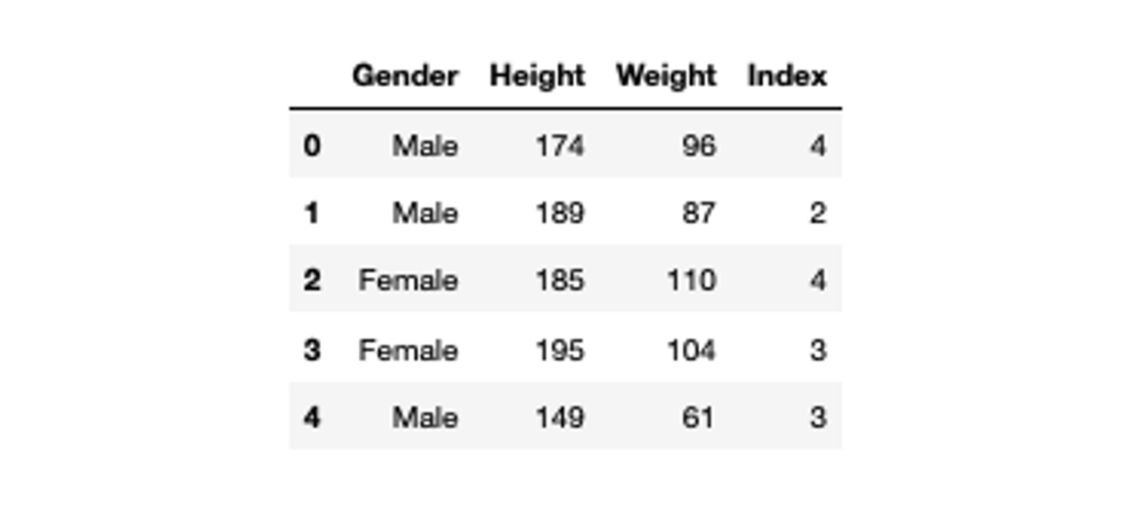

Most algorithms need numerical data, so we need to convert the Gender column to numerical.

# convert gender to binary values
bmi_data['Gender'] = bmi_data['Gender'].map({'Male':0, 'Female':1})
bmi_data.head()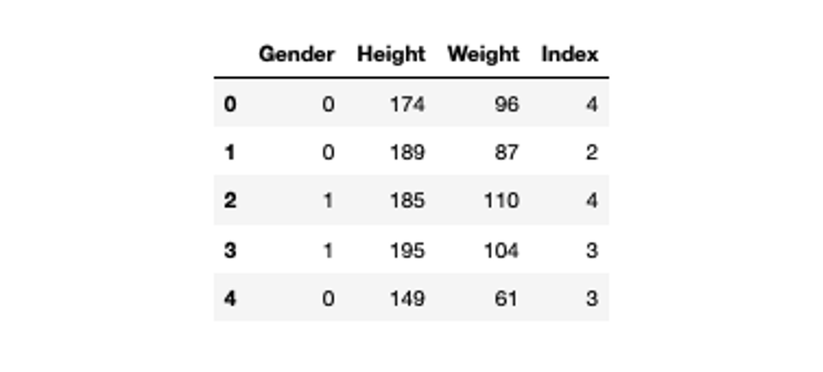

Now, let’s go over the methods of detecting the multicollinearity in the data.

Descriptive Methods

Variance Inflation Factor (VIF)

The most straightforward way to detect multicollinearity in data is using a metric called Variance Inflation Factor (VIF). VIF identifies the correlation between independent variables and quantifies the strength of this correlation. It starts with a value of 1 that indicates no correlation between independent variables. Values between 1 and 5 indicate a moderate correlation that likely has little impact. A value greater than 5 represents a critical level of correlation in variables.

Note: VIF can not be applied to the categorical data. Also, the upper limit to decide if the features are correlated or not totally depends on your data, sometimes this value is set to 10.

The statsmodel library in Python provides the implementation of VIF. It can be downloaded with PIP as follows:

$ pip install statsmodels

You need to import the dependency for VIF in your notebook as follows:

from statsmodels.stats.outliers_influence import variance_inflation_factor

Then, to make the process more interpretable you can create a dataframe that defines all the independent variables.

# columns to check VIF for
X = bmi_data[['Gender', 'Height', 'Weight', 'Index']]

To store the VIF value we will create an empty dataframe and will iterate over each variable in our data to calculate the VIF using the variance_inflation_factor() method.

# create an empty dataframe
vif = pd.DataFrame()

# copy all the features of X in vif dataframe
vif["features"] = X.columns

# calculate VIF for all the variables
vif["VIF Factor"] = [variance_inflation_factor(X.values, i) for i in range(X.shape[1])]
vif

As you can see, the VIF values for Height, Weight, and Index are extremely high. This indicates that there lies a strong correlation in this dataset.

Correlation Matrix

Another simple method of detecting the multicollinearity in your dataset is to use the correlation matrix. This matrix comprises different correlation coefficients that represent the correlation of one predictor variable with other predictor variables in the data. An absolute value > 0.7 represents the strong correlation between the variables. Also, the correlation of any predictor variable with itself is always 1.

Note: Value of 0.7 is not fixed you can always decide on this threshold based on your data.

There are various methods to calculate this correlation matrix but the most popular and regularly used one is the Pearson Correlation method. The Pandas library already has a built-in method corr() that calculates the correlation matrix on the given dataframe.

# calculate correlation values
correlation_matrix = bmi_data.corr()
correlation_matrix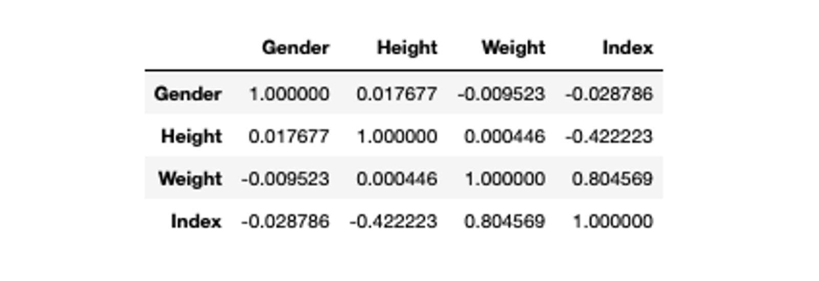

As you can observe Weight and Index columns have a correlation value of 0.8 which represents a strong correlation and also varifies our results from the VIF method.

Graphical Methods

Heatmaps

This is not a specific method to detect the multicollinearity instead it helps to easily visualize the correlation results. The Seaborn library in Python provides the heatmap() method for creating the heatmaps using the correlation matrix.

# set figure size
plt.figure(figsize=(6,5))

# plot correlation matrix
sns.heatmap(correlation_matrix, annot=True)

# set the title
plt.title('Correlation Matrix')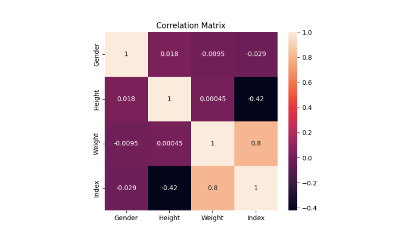

Now correlation values are easily visualizable and interpretable with a simple graph.

Clustermaps

Clustermaps are modifications to the heatmaps that represent a hierarchical cluster of different rows and columns in the data.

They are specially used to represent the correlation of different predictor variables in the data as they can cluster the highly correlated ones into one group. The Seaborn module provides the clustermap() method to create cluster maps in Python.

# set figure size
plt.figure(figsize=(6,5))

# plot correlation matrix
sns.clustermap(correlation_matrix, annot=True)

# set plot title
plt.title('Correlation Matrix')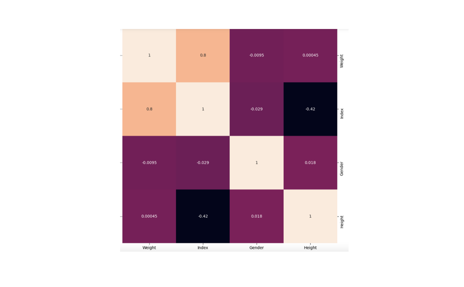

You can check in the above graph that the highly correlated variables are clustered together.

Regression-Based Methods

Eigenvalues

Eigenvalues can be used to check the presence of multicollinearity in the data as they capture the variance in the data. The smaller eigenvalues represent the instability in the estimation of the regression coefficient and high multicollinearity among the predictor variables. Usually, a value less than 1 (closer to 0) indicates high collinearity in the data while a value greater than 1 represents moderate or no collinearity.

Note: There is not a fixed predefined threshold that tells us the degree of multicollinearity. The rule of thumb is, that if one of the eigenvalues in your data is much less than the others then there could be multicollinearity in the data.

To calculate the eigenvalues, you need to start by calculating the correlation matrix of the predictor variables. And the Numpy library provides the eigvals() method to calculate eigenvalues.

# Calculate the correlation matrix
correlation_matrix = bmi_data.corr()

# Calculate eigenvalues
eigenvalues = np.linalg.eigvals(correlation_matrix)
eigenvalues

Here, we can see that the second value is much lower than the others, suggesting multicollinearity.

Condition Index

An alternative to VIF is the conditional index method. This method shows the degree of multicollinearity for the predictor variables.

It is calculated as the square roots of the ratios between the greatest and subsequent eigenvalues in the data. Although there are no standard values that tell how severe the correlation is, generally a value between 5 and 10 represents a weak correlation. While a value greater than 30 represents a strong correlation.

To calculate the condition index you can use the Numpy library of Python. To begin with this metric, you need to first calculate the correlation among variables then calculate the eigenvalues from the correlation matrix and finally calculate the square root of the the ratios between greatest and subsequent eigenvalues.

# Calculate the correlation matrix
correlation_matrix = bmi_data.corr()

# Calculate eigenvalues
eigenvalues = np.linalg.eigvals(correlation_matrix)

# Calculate the condition index
condition_index = np.sqrt(max(eigenvalues) / eigenvalues)
print(f"Condition Index: {condition_index}")

Interestingly, this method doesn’t show a strong correlation. Not all methods to detect multicollinearity will work equally well or provide consistent results on every dataset. The effectiveness of multicollinearity detection methods can vary depending on several factors, including the characteristics of the dataset and the nature of the multicollinearity present.

Remedying Multicollinearity

Now that you are aware of different methods of detecting multicollinearity in the data, let’s discuss methods that can help you get rid of it when needed.

Dropping Redundant Variables

The straightforward method to deal with multicollinearity is removing one or more correlated predictor variables from the dataset. Although this method seems easy, it requires the domain knowledge and a clear objective. If you are not aware of the business use case for which you are using the data, you might not be able to figure out which feature to keep (meaningful feature) and which one to get rid of. This is a core part of feature selection.

You can use the drop() method from the Pandas to drop one or more variables from the data.

# Remove highly correlated independent variables
bmi_data_2 = bmi_data.drop(['Index', 'Weight'], axis=1)

# calculate VIF
vif = pd.DataFrame()
vif["VIF Factor"] = [variance_inflation_factor(bmi_data_2.values, i) for i in range(bmi_data_2.shape[1])]
vif["features"] = bmi_data_2.columns
vif

After dropping the highly correlated variable, the VIF values have come into place.

Principal Component Analysis (PCA)

Although dropping the correlated features seems to be simple it can lead to loss of crucial information that results in poor estimation of the parameters in models, so you can not always trust it.

There is one more widely used concept, Principal Component Analysis (PCA), for removing the multicollinearity in data. PCA helps in remedying multicollinearity by combining one or more correlated predictor variables into a single or multiple variables known as principal components. To do this it uses covariance metrics, eigenvalues, and eigenvectors combined. This concept is also a cure for the curse of dimensionality where you have a lot of features in your dataset and can’t work through them. To learn more about PCA, you can refer to this article.

The scikit-learn library of Python provides the implementation of PCA and it can be downloaded with PIP as follows:

$ pip install scikit-learn

The fit_transform() method of PCA helps you to convert the highly correlated features into single or multiple features. It typically means that you are using the same data for training and inference of PCA.

from sklearn.decomposition import PCA

# Use PCA to combine highly correlated independent variables
pca = PCA(n_components=1)

# create a copy of original data
data = bmi_data.copy()

# compute PCA for correlated columns
data['pca'] = pca.fit_transform(bmi_data[['Index', 'Weight']])

# drop the correlated columns
data = data.drop(['Index', 'Weight'], axis=1)
data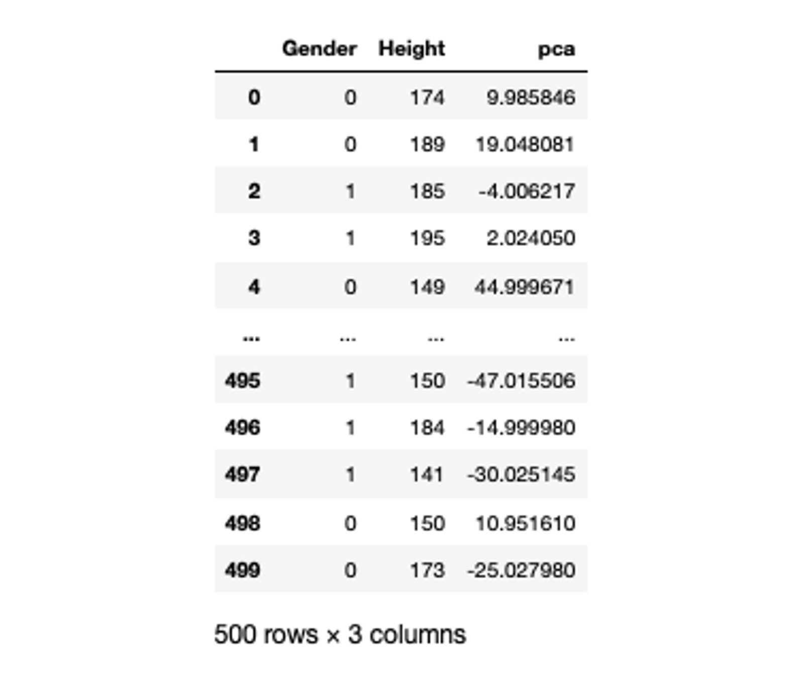

Once the new column is generated, you can get rid of the highly correlated variables and use the newly generated one. The argument n_components in PCA tells the algorithm to produce N number of principal components.

Ridge Regression

It is not always necessary that you have to make changes to the data to deal with multicollinearity. You can also use machine learning models like Ridge Regression, Lasso Regression, or Elastic Net Regression.

Ridge regression, for example, helps remedy multicollinearity by introducing a regularization term that encourages smaller coefficient values, effectively reducing the sensitivity of the model to correlated predictor variables. This regularization leads to more stable and interpretable regression coefficients and can improve the overall performance of the model in the presence of multicollinearity.

The scikit-learn library provides an implementation of almost all kinds of regression algorithms including ridge regression. You simply need to segregate your independent and dependent variables and pass them to the fit() method of the ridge regression.

from sklearn.linear_model import Ridge

# create dependent and independent variables
X = bmi_data.drop('Index', axis=1)
y = bmi_data['Index']

# Use Ridge regression to remedy multicollinearity
ridge = Ridge(alpha=0.1)
ridge.fit(X, y)

This will help you give the best regression coefficients and the model will be able to produce better predictions.

Other Methods

Apart from the methods mentioned above, you can also use feature selection methods for different numerical and categorical variables to select the best parameters that in turn reduce the effect of multicollinearity. In some scenarios, scaling different predictor features (feature scaling) on the same scale may reduce the effect of collinearity.

Note: You need to be aware that not all methods will work the same on your dataset as treating the multicollinearity always depends on the type, source, and nature of it.

The code used in this article can be found here.

Fixing multicollinearity

Your choices for detecting and fixing multicollinearity algorithms depends on the type of data and business use case that you are working on. Sometimes you may need to use a combination of them to make data analysis more effective.

But it is worth going through this process to ensure the validity, reliability, and accuracy of your model. When the model accurately reflects the individual contribution of each variable, it results in more robust and reliable predictions, allowing for informed decision-making. Navigating through multicollinearity ensures that the insights gleaned from the model are clear, precise, and free from the distortion that can arise from overlapping variables.

Learn more about what causes multicollinearity and what are its different types to easily understand which approach may work out best for you.