Unveiling patterns in unlabeled data with k-means clustering

Data clustering algorithms are a machine learning technique that can group similar data points, even if they are not labeled.

k-means clustering is a core data clustering algorithm used in everything from market segmentation and image compression to customer profiling and anomaly detection. Let’s see how it works so you can start to use it in your work too.

Fundamentals of K-Means Clustering

At its core, K-means clustering is a simple but effective algorithm for partitioning unlabelled data into a predefined number of clusters to uncover hidden patterns in unlabelled data. It belongs to the family of unsupervised learning algorithms which means it doesn’t require pre-labeled data for training. K-means takes a collection of data points and divides them into a ‘K’ number of clusters. The algorithm does this by repeatedly assigning data points to the nearest cluster center and recalculating the center based on newly formed points. This process continues until a significant change is found in cluster center change where the algorithm successfully concludes the grouping of data points into K clusters.

How K-Means Works?

Imagine you have a collection of data points scattered in space, and you want to group them into K clusters, below are the steps for how the K-Means algorithm accomplishes it.

1. Initialization: K-means randomly places K number of centroids in the data space. This center defines the starting points for the clusters.

• Assignment: K-means assign each data point to the nearest cluster centroid based on distance metric, typically Euclidian distance, Manhattan distance, or Cosine similarity. This step is most crucial as it determines which cluster each data point belongs to.

• Updating the Cluster Centers: After assigning all data points, the algorithm recalculates the centroid by taking the mean of all data points to that centroid’s cluster reducing the intra-cluster variance in relation to the previous step. These new centers represent the average location of each data point in each cluster.

• Iterative Process: Step 2 and Step 3 are repeated iteratively. Data points are reassigned to the nearest cluster, and cluster centers are updated accordingly in each iteration until cluster centers no longer change significantly or the pre-defined number of iterations is reached.

Key Parameters of Clustering

Now before performing the K-means algorithm, you must know the key parameters that affect its performance.

• K (Number of Clusters): The number of clusters you want to identify needs to be defined before running the algorithm. Selecting the right K is often a challenging task and requires domain knowledge or techniques like the Elbow method to make an informed choice.

• Initialization Methods: The way you initially position the cluster centers influences the outcome. Common methods include random initialization, k-Means++, and others. Proper initialization can improve the quality of clusters.

Unveiling Patterns in Unlabeled Data with K-Means Clustering

Let’s work through an entire k-means clustering problem. You can see the entire code in our Hex notebook.

Let’s install our dependencies first.

# using PIP
pip install pandas numpy matplotlib scikit-learn

The Pandas and Numpy libraries help load and preprocess the data, Matplotlib helps us visualize the results and finally, the Scikit-learn library helps us to perform the K-Means clustering on unlabelled data.

Preprocessing Unlabeled Data

The first step is to load the required dependencies that we will be using for loading data, visualizing results, and performing k-means clustering.

# data loading dependencies
import numpy as np
import pandas as pd

# visulaization dependency
import matplotlib.pyplot as plt

# data preprocessing dependencies
from sklearn.datasets import load_iris
from sklearn.preprocessing import StandardScaler
from sklearn.decomposition import PCA
from sklearn.metrics import silhouette_score

# k-means dependency
from sklearn.cluster import KMeans

Loading Public Dataset

For this demo, you will be working on the Iris Dataset. The iris dataset is a classic machine-learning dataset that contains data for sepal length, sepal width, petal length, and petal width of iris flowers. The dataset is a good choice for exploring clustering algorithms because it has a small number of features clustered into three groups.

# load the Iris dataset
iris = load_iris()

# create a Pandas Dataframe from the Data
df = pd.DataFrame(iris['data'], columns=iris['feature_names'])

# print the DataFrame
df.head()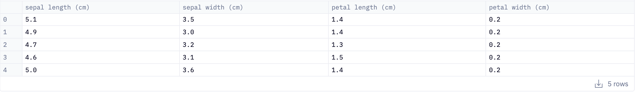

Data Cleaning

Data cleaning is a process of identifying irregularities and correcting errors in the data. Irregularities involve handling missing values, and invalid data points, addressing outliers, and correcting typos. For the Iris dataset the data is clean but Below is a simple example of how you can perform data cleaning.

# remove data points with missing values
df.dropna(inplace=True)

# correct typos in the feature names
df.columns = ['sepal_length', 'sepal_width', 'petal_length', 'petal_width']

# fill in missing values with the mean value for that feature
df.fillna(df.mean(), inplace=True)

Data Transformation

Data transformation is the process of converting data into a format that is more suitable for machine learning algorithms. This may include scaling, converting categorical data into numerical features, and creating a new feature from existing features, etc. For Iris data, we will apply the standard scaling on the data.

# scale the data using the StandardScaler
scaler = StandardScaler()
df_scaled = scaler.fit_transform(df)
df_scaled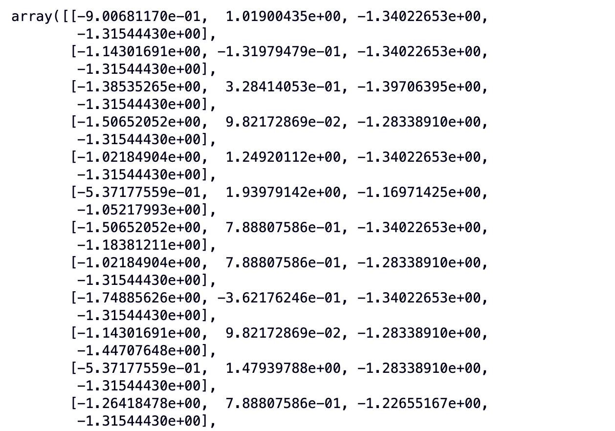

In most of the real-world use cases, you might face the curse of dimensionality. To deal with it, there are several techniques available like PCA (Principal component analysis) which works by identifying the principal component of the data and helps with feature selection. The iris dataset does not require dimensionality reduction (due to the lower number of features) but below is the demo snippet of how you can use PCA to reduce the dimensionality of the iris dataset or any other.

# reduce the dimensionality of the data using PCA
pca = PCA(n_components=2)
df_pca = pca.fit_transform(df_scaled)
df_pca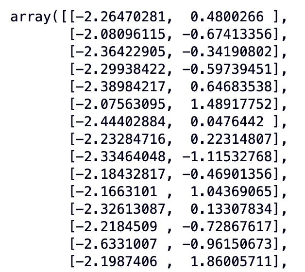

Note: We will still use the original data with 4 features for K-means clustering.

Selecting an Optimal Value of K

Some factors can challenge the efficacy of the final output of the k-means algorithm, and one of them is finalizing the number of clusters (k). Selecting the lower number of clusters can result in the algorithm in an underfitting condition while the higher number of clusters can overfit the model. Hence, selecting the optimal value of k ensures clustering results are accurate and meaningful.

The parameters and similarity metrics used in the clustering process determine the ideal number of clusters. To find the best value of k you need to run k-means for a range of values and compare the outcomes. Different techniques do the same for you. In this section, you will see different techniques to estimate the best value of K.

Elbow Method

The Elbow method is a commonly used metric to compare the results across different k values and find the optimal one. When the number of clusters (k) is increased the distance from the centroid to the data point will be decreased and will reach a point where k is the same as the number of data points. Thus we use the mean of the distance of centroids. Plotting the mean distance, we search for the elbow point in the Elbow technique when the rate begins to gradually drop. This is generally considered the optimal value of K. It is an iterative process where K-means will be performed on the range of values of k, and plot each of these points to find the point where the mean distance suddenly falls.

The scikit-learn library of Python provides the implementation of K-means. And you can perform the elbow method analysis as follows.

# calculate the inertia (within-cluster sum of square) for different values of K
inertias = []
for k in range(1, 11):
	kmeans = KMeans(n_clusters=k)
	kmeans.fit(df_scaled)
	inertias.append(kmeans.inertia_)

# plot the inertia vs K
plt.plot(range(1, 11), inertias, marker='o', linestyle='--')
plt.xlabel('K')
plt.ylabel('Inertia')
plt.title('Elbow Method for Iris Dataset')
plt.show()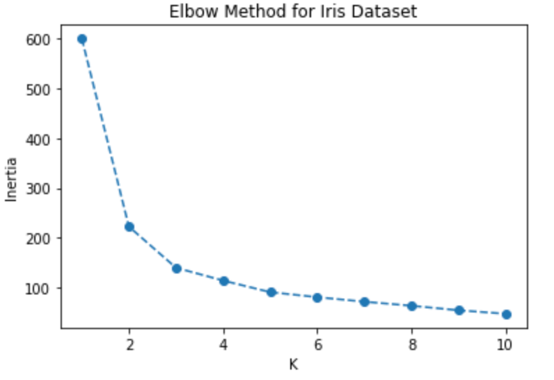

By observing the above elbow curve the optimal value of K can be between 2 to 4 because after 4 the mean distance gradually starts to decrease.

Silhouette Score

Determining the Elbow point can be a challenging task but there are other techniques to find the optimal value of k, and one of them is the Silhouette Score. An indicator of how closely each data point is grouped is the Silhouette score. By comparing the degree of similarity between each data point within a cluster and other clusters, it is used to assess the quality of clusters. It accepts the values between -1 and 1, with a higher score indicating better clustering. Below are the steps on how to determine Silhouette scores.

1. For a range of k values, calculate the K-means.

2. For each value of k find the average silhouette score.

3. For every value of k, plot the collection of silhouette scores.

4. Select the number of clusters when the score is maximum.

# calculate the silhouette score
silhouette_scores = []
for k in range(2, 11):
	kmeans = KMeans(n_clusters=k)
	kmeans.fit(df_scaled)
	silhouette_scores.append(silhouette_score(df_scaled, kmeans.labels_, metric = 'euclidean'))

# plot the silhouette score vs K
plt.plot(range(2, 11), silhouette_scores)
plt.xlabel('K')
plt.ylabel('Silhouette Score')
plt.title('Silhouette Score for Iris Dataset')
plt.show()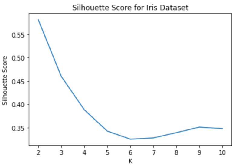

Using the above analysis you can choose K’s optimal value as 2 because the average silhouette score is higher.

Gap Statistics

Gap statistics is a more polished method for selecting the best value of k. The method compares the total within-cluster sum of squares of data to data distribution. And the optimal value is that minimizes the gap between the WCSS of the data and the WCSS of reference distribution.

# calculate the gap statistics for different values of K
gap_statistics = []
for k in range(2, 11):
	kmeans = KMeans(n_clusters=k)
	kmeans.fit(df_scaled)
	gap_statistics.append(silhouette_score(df_scaled, kmeans.labels_))

# plot the gap statistics vs K
plt.plot(range(2, 11), gap_statistics)
plt.xlabel('K')
plt.ylabel('Gap Statistic')
plt.title('Gap Statistics for Iris Dataset')
plt.show()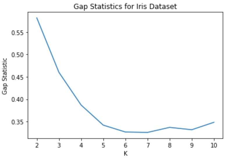

Running K-Means Clustering

Once you have the optimal value of k, you are ready to run the k-means clustering algorithm. The technique works by iteratively allocating data points to clusters and updating the cluster centroids.

The first step is to define the number of clusters (k) that you have identified using one of the methods mentioned above.

# initialize the cluster centroids
kmeans = KMeans(n_clusters=3, init='random')

In the above code, we have created an object of the KMeans() method where the number of clusters is 3 and we are using the random initialization method. Next, let’s train the K-means clustering on our Iris data.

# train the model
kmeans.fit(df_scaled)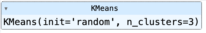

This is it, that is all you need to do for running the k-mean clustering algorithm on unlabeled data.

Analyzing Cluster Results

Once you have successfully run k-means clustering on your data and determined the optimal number of clusters, the next step is analyzing the algorithm performance.

Cluster Interpretation

It is a process of understanding what each cluster represents in a k-means clustering algorithm. This can be done by looking at the data points in each cluster, the size of each cluster, and the relationship between the clusters. For example, in our Iris dataset, you can find the average values of the features within each cluster to interpret what each cluster represents.

To do so let’s create a dataframe from our scaled features as follows:

# create a dataframe to analyze results
df_scaled_df = pd.DataFrame(df_scaled)
cluster_labels = kmeans.labels_

Once done, you can analyze the results as follows:

# calculate the mean and standard deviation of each feature for each cluster
cluster_means = df_scaled_df.groupby(cluster_labels).mean()
cluster_stds = df_scaled_df.groupby(cluster_labels).std()

# print the cluster means and standard deviations
print(cluster_means)
print(cluster_stds)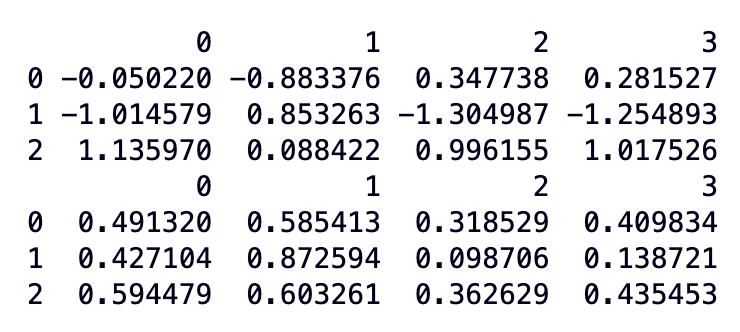

As you can observe:

• Cluster 0 has the lowest mean values for all four features. This suggests that Cluster 0 contains the smallest Iris flowers.

• Cluster 1 has intermediate mean values for all four features. This suggests that Cluster 1 contains medium-sized Iris flowers.

• Cluster 2 has the highest mean values for all four features. This suggests that Cluster 2 contains the largest Iris flowers.

Visualizing Clusters

Visualization is a powerful method to understand the cluster results. You can create different visualizations to gain different conclusions. Some popular techniques include scatter plots, parallel coordinates, or T-SNE for dimensionality reduction.

# create a list of colors for each cluster
cluster_colors = ['red', 'green', 'blue']

# plot the data points colored by cluster
for i in range(len(cluster_labels)):
	plt.scatter(df_scaled_df.iloc[i, 0], df_scaled_df.iloc[i, 1], c=cluster_colors[cluster_labels[i]], s=50)

plt.xlabel('Sepal Length')
plt.ylabel('Sepal Width')
plt.title('Iris Dataset Clusters')
plt.show()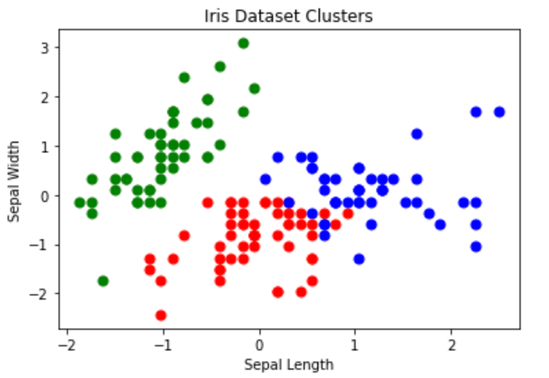

Evaluating K-Means Clustering

Evaluating the performance of the algorithm is important and can be done using a variety of evaluation metrics such as the Silhouette score, Dunn index, etc. These metrics help determine how well the data points are grouped and how distinct clusters are from each other.

# calculate the silhouette score
silhouette_score = silhouette_score(df_scaled, cluster_labels)

# print the silhouette score and the inertia
print('Silhouette score:', silhouette_score)

As you already know the value of silhouette score varies from -1 to 1, 1 being the best. Our algorithm provides a score of 0.45 which is just good enough.

This is it, now you are ready to work on any unlabelled dataset to find patterns in it. You can find the code used in this article here.

The Power of k-means Clustering

Finding meaningful patterns in vast seas of information is imperative. With k-means clustering, businesses like e-commerce platforms can sift through the noise, categorizing vast customer datasets into actionable segments. By understanding and grouping similar data points, brands can tailor marketing campaigns, offer recommendations, and create personalized experiences, all without needing explicit labels. While it's just one tool in the vast arsenal of machine learning, k-means clustering stands out for its simplicity, efficiency, and adaptability. As you dive into your data challenges, remember the Trevors out there—finding them efficiently could be the key to your next big success.