Using Autoencoders for Feature Selection

Machine learning models work most effectively when they are trained on high-quality data. The quality of this data is determined by the quality of its features.

So features need to be relevant, informative, and non-redundant for the model to learn effectively. Feature selection is the process of identifying the most essential features in the dataset that lead to the optimal model performance in machine learning. It is critical for improving model performance, avoiding any confusion for models to identify relationships between features, reducing computational complexity, and improving interpretability.

Although there are different techniques for feature selection (Filter methods, wrapper methods, and Embedded Methods), one remarkable approach that has gained appreciation in recent years is the use of autoencoders. Autoencoders are a class of artificial neural networks used in tasks like data compression and reconstruction. In this article, we will delve into the world of autoencoders, explore their architecture, and discuss autoencoders as a powerful tool for feature selection.

The Basics of Autoencoders

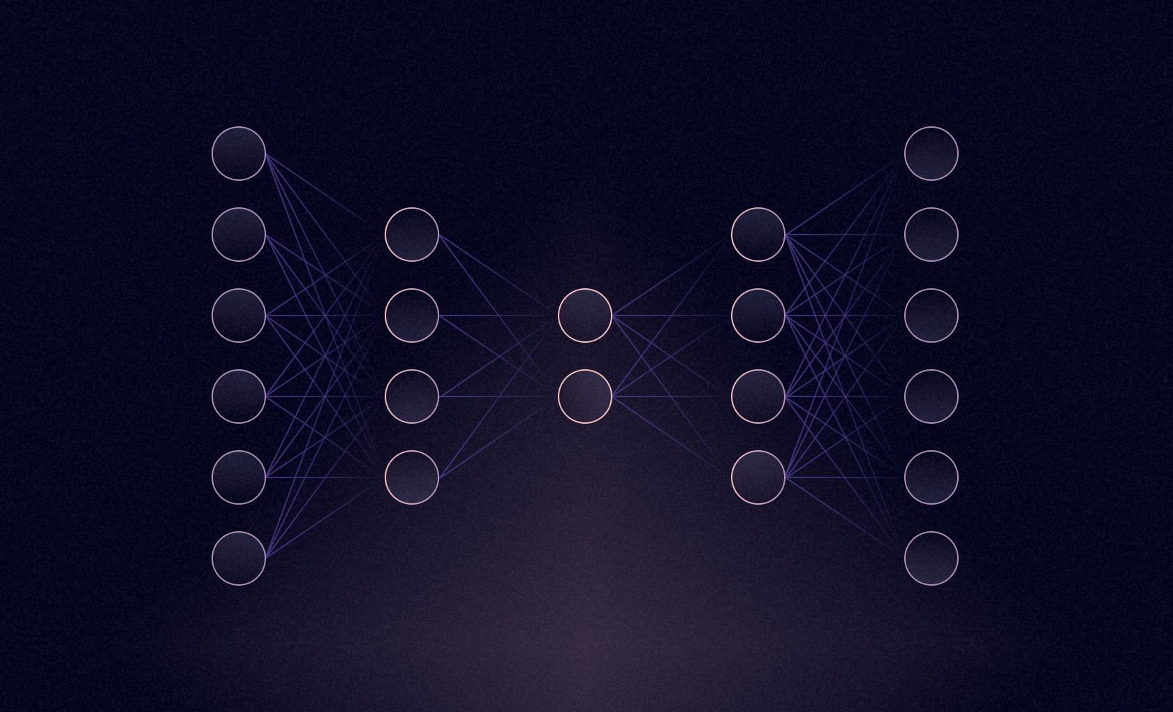
Autoencoders are neural network models that are trained to reconstruct the input data. They do this by learning a compressed representation of data, called the latent space, and then reconstructing the data from the latent space. For example, if you have an image of a cat, the autoencoder learns to compress the picture into a smaller, more abstract representation, such as a set of numbers, and then reconstruct the picture from this compressed representation.

Architecture of Autoencoders

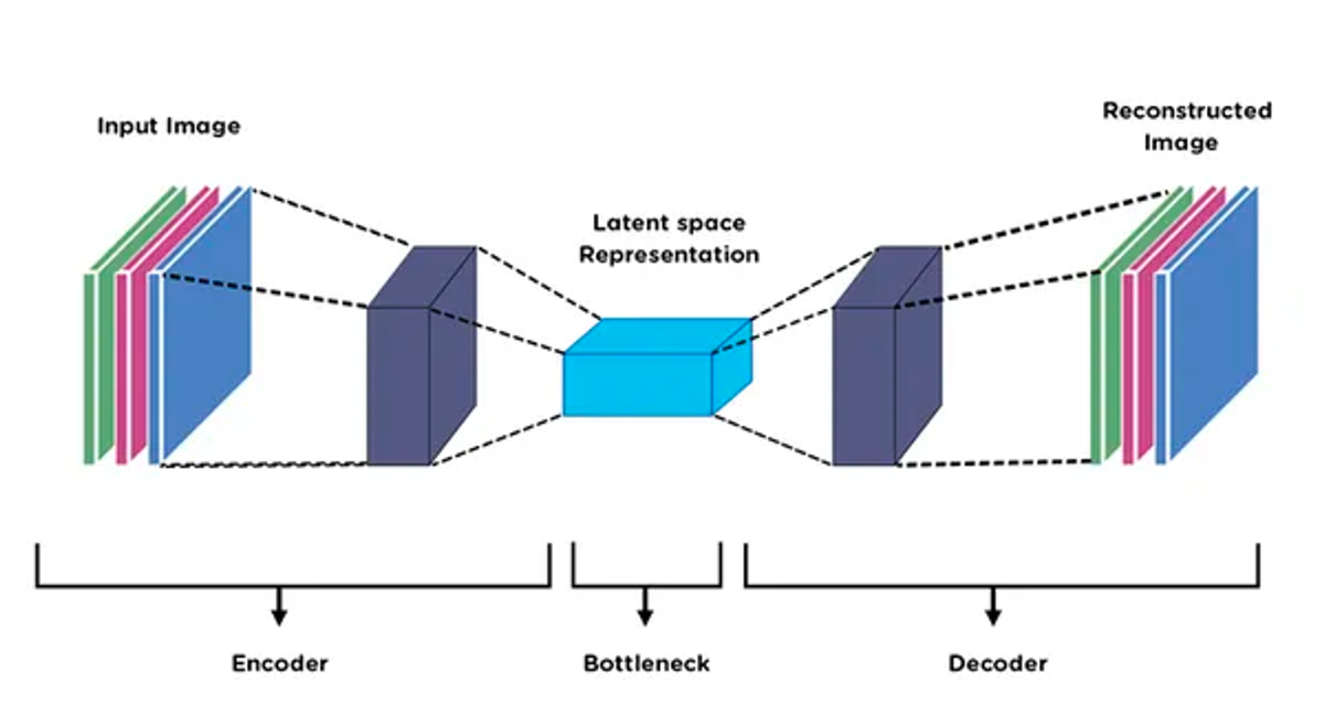
The architecture of the autoencoder is the critical aspect of its functionality. It consists of several components that work to compress and reconstruct the input data.

The key components are:

Input Layer

The input layer is where the original data is fed to the autoencoder. The input layer should have the same number of neurons as the number of features in the data.

Encoder

The encoder contains a series of encoding layers (hidden layers) where each layer consists of a set of neurons responsible for compressing the input data into latent space by reducing the dimensionality of data. Neurons in the first encoding layer capture simple, low-level features, while deeper layers capture more abstract and complex features. Each layer of the encoder uses a non-linear activation function to transform its input. The encoder’s final layer, known as the bottleneck layer, has a significantly small number of neurons compared to the input layer. This layer represents the compressed form of input data.

Latent Space

The bottleneck layer serves as the latent space. It encodes the most salient information from input data in a reduced-dimensional format. The compressed representation is a vital part of the autoencoder that captures the important features while discarding the non-relevant ones.

Decoder

The decoder contains a symmetric set of decoding layers that reconstruct the original data from the latent space (encoded form). Similar to encoding layers each decoding layer consists of neurons that gradually expand the dimensionality of data. The last decoding layer produces the output that should closely resemble the original input data.

Output Layer

The output layer is where the reconstructed data is concluded by the autoencoder. The output layer should have the same number of neurons as the number of features in the input data.

One of the best applications of the autoencoder is dimensionality reduction, which is the process of reducing the number of features in a dataset while still retaining as much useful information as possible. Training the autoencoder network to compress and decompress the data, significantly reduces the dimensionality of the dataset by dropping the non-relevant features. Autoencoders can also learn non-linear relationships between input features, so can perform non-linear dimensionality reduction. Hence it not only simplifies the data but also serves as a powerful feature selection mechanism.

Autoencoders for Feature Selection

Autoencoders have a unique approach to feature selection, addressing several challenges, and limitations associated with conventional methods.

Challenges and Limitations of Traditional Feature Selection Methods.

Traditional feature selection methods like filter methods, wrapper methods, and embedded methods simplify complex datasets for machine learning models and are simple to understand and implement. However, they come with some set of drawbacks.

• Lack of Data Understanding: Filter methods that use some statistical measure for feature selection lack in deeper understanding of data which may lead to the removal of potentially relevant features.

• Computational Intensity: Wrapper methods like forward selection or backward elimination require training of the network model multiple times, making them computationally intensive and impractical to use for large datasets.

• Overfitting Risks: These methods may lead to overfitting when trying to optimize the model performance, as they may select the features that are beneficial but are not generalizable.

• Curse of Dimensionality: Embedded methods, while integrating feature selection into model training, can struggle with high-dimensional data, leading to increased computational complexity.

• Manual Feature Engineering: Many traditional methods rely on domain knowledge and require manual feature engineering which makes them less adaptable to diverse datasets.

Motivation Behind Using Autoencoders

The adoption of autoencoders for feature selection arises from several compelling motivations

• Automated Feature Extraction: Autoencoders use deep neural network to automatically learn and extract meaningful features from data which eliminate the need for manual feature engineering.

• Non-linearity Handling: Autoencoders can capture complex, non-linear relationships from data that traditional methods fail to detect.

• Dimensionality Reduction: Autoencoder compresses data into lower dimensional latent space with the help of encoding layers to address the curse of dimensionality.

• Data Reconstruction: Autoencoders are designed to reconstruct data accurately. It determines the important features that are necessary to perform the predictive task and retain those features, performing feature selection.

• Adaptability: Autoencoders are versatile and can be applied to different types of datasets including images, audio, text, and numerical data which enable them to work on multiple applications.

• Transfer Learning: There are various pre-trained autoencoders present that can be fine-tuned for specific tasks which provides a transfer learning advantage in feature selection.

Autoencoders can be used as unsupervised feature selection tools by identifying the latent space representations that are most important for reconstructing the input data. These latent space representations can be used to select a subset of features for training an AI model. This can improve the performance of the AI model by reducing the noise in the data and by focusing on the most essential features.

Steps to Use Autoencoders For Feature Selection

Let’s go through an example of using autoencoders for feature selection. We will be using the publicly available Iris dataset to demonstrate how autoencoders can efficiently select important features for predictive modeling. This dataset consists of the measurement of four features (sepal length, sepal width, petal length, and petal width) of three different species of iris flowers. Each species is labelled properly making it suitable for supervised learning tasks.

You can see the entire Hex notebook here:

Install and Load Dependencies

For this section, you will need some of the core computational libraries for Python: Numpy, Pandas, SKLearn, and Keras. These libraries can be installed through a terminal with Python Package Manager (PIP) as follows:

$ pip install pandas numpy scikit-learn keras

Once the libraries are installed, you need to import them into Hex:

# Import necessary libraries for loading and processing data
import numpy as np
import pandas as pd
from sklearn.preprocessing import StandardScaler
from sklearn.model_selection import train_test_split
from sklearn.datasets import load_iris

# Import Keras for implementing autoencoders
import keras
from keras.models import Sequential
from keras.layers import Input, Dense

Data Preprocessing

Before diving into feature selection with autoencoders, the next step is to load and preprocess the data to make it ready to feed to the model.

In this step, you will load the iris dataset and standardize the dataset to ensure all features have a mean of 0 and a standard deviation of 1. Standardization helps autoencoders converge faster during training and ensures that features are on a similar scale.

# load the Iris dataset
iris = load_iris()
data = iris.data
target = iris.target

# Standardize the data
scaler = StandardScaler()
data = scaler.fit_transform(data)

# Split the data into training and test sets
X_train, X_test, y_train, y_test = train_test_split(data, target,                                                    test_size=0.2, random_state=42)

In the above code, we first load the data using the load_iris() method from sklearn. Then we apply the StandardScaler() method to bring all the features to the same scale. Finally, for the experiment, we divide the data into a training and testing set.

Building an Autoencoder

The next step is to construct an autoencoder, which is a neural network that will learn to compress and reconstruct the input data. The autoencoder architecture layers are defined below.

• Input Layer: Matches the number of features in the dataset.

• Encoding layer: Reduces the dimensionality of data.

• Decoding layer: Reconstructs the input from the encoded representation.

Keras library of Python provides the implementation of all these layers of autoencoder.

# Define the autoencoder architecture
input_dim = X_train.shape[1]
encoding_dim = 2

# Set the encoding dimension
input_layer = keras.layers.Input(shape=(input_dim,))
encoder = keras.layers.Dense(encoding_dim, activation="relu")(input_layer)
decoder = keras.layers.Dense(input_dim, activation="sigmoid")(encoder)
autoencoder = keras.Model(inputs=input_layer, outputs=decoder)

# Compile the autoencoder
autoencoder.compile(optimizer='adam', loss='mse')

# Summary of the autoencoder architecture
autoencoder.summary()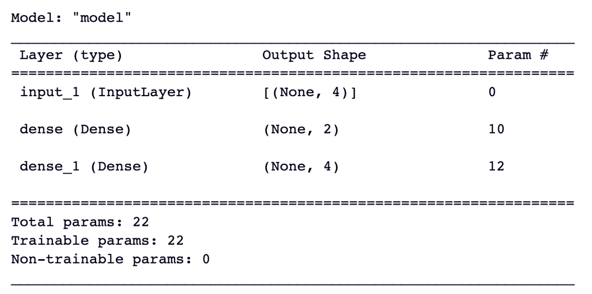

In the above code, we first define the input dimension and the dimension of the encoder. Then we created three different layers using the keras.layers module that correspond to the input layer, endcoding layer, and decoding layer. We are using the adam optimization algorithm and mean squared error loss for training the autoencoder. Finally, if you want to check the whole architecture, you can use the summary() method from keras.

Training the Autoencoder

After constructing the complete neural network model of the autoencoder it’s time to feed the input data to the model and train the model on the iris dataset. Using this process autoencoder network can compress and learn important features from the dataset.

# Train the autoencoder
autoencoder.fit(X_train, X_train, epochs=100, batch_size=32, shuffle=True, validation_data=(X_test, X_test))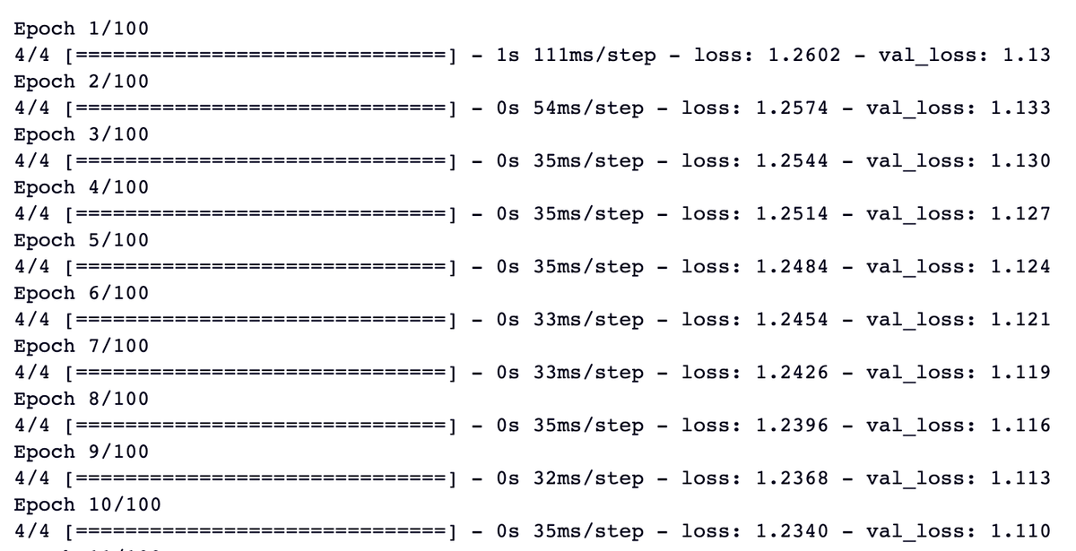

We call the fit()method from Keras to train the model. This method requires the Independent and dependent variables (training data), number of epochs, batch size, and other optional parameters. Once you run this code, the model will start training for the given number of epochs.

Note: Batch size and number of epochs depend on the dataset that you are using for training.

Extracting Important Features

After training the Autoencoder, you can extract the important features that the encoder has found useful. These features represent the compressed version of input data and can be used as selected features.

# Use encoder part of the autoencoder for feature selection
encoder = keras.Model(inputs=autoencoder.input, outputs=autoencoder.layers[1].output)
encoded_features_train = encoder.predict(X_train)
encoded_features_test = encoder.predict(X_test)

# Display the shape of extracted features
print("Encoded Features Shape (Train):", encoded_features_train.shape)
print("Encoded Features Shape (Test):", encoded_features_test.shape)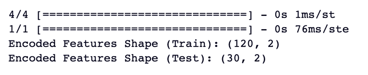

Combining Selected Features with a Predictive Model

Finally, you can integrate the selected features with the predictive model (any relevant machine learning algorithm) like logistic regression to evaluate the effectiveness of feature selection using autoencoders.

# Import a predictive model (e.g., logistic regression)
from sklearn.linear_model import LogisticRegression
from sklearn.metrics import accuracy_score

# Fit a logistic regression model using the selected features
model = LogisticRegression()model.fit(encoded_features_train, y_train)

# Make predictions on the test set
y_pred = model.predict(encoded_features_test)

# Calculate accuracy
accuracy = accuracy_score(y_test, y_pred)
print("Accuracy with Selected Features:", accuracy)

By following the above steps you can successfully implement the autoencoder for feature selection on any dataset for the specific problem statement you are dealing with.

This method allows us to select the best features that highly dominate to target variable and then integrate these features with a machine learning algorithm to build the well generalized model with good performance while reducing dimensionality and computational complexity.

Challenges and Limitations of Using Autoencoders as Feature Selectors

Autoencoders are a powerful tool for feature selection and data compression, but they are not without challenges and limitations. It is important to be aware of these factors to make informed decisions when using autoencoders in solving any machine learning problem statement.

Overfitting and Underfitting Issues

Autoencoders are prone to overfitting, a common problem in deep learning. Overfitting occurs when the autoencoder model learns the training data too well capturing noise and irregularities in data and then is unable to generalize to new data or does not perform on any new data with expected performance. Underfitting occurs when the autoencoder does not learn the training data well enough and is unable to reconstruct the input data accurately.

To avoid overfitting and underfitting, it is important to carefully choose the above architecture of the autoencoder and to address it using techniques like dropout, early stopping, and regularization techniques.

Interpreting Feature Importance with Autoencoders

Autoencoders are also known as black-box models, making it difficult to interpret the significance of selected features. Unlike traditional feature selection methods that provide explicit feature rankings, autoencoders learn a compressed representation of data which can make it difficult to understand which features are the most important.

To interpret the feature importance from autoencoders use a technique called latent space analysis. It involves looking at the relationships between features in the latent space. Features that are highly correlated in latent space are likely to be important.

Handling High-Dimensional Data

Autoencoders can be used to handle high-dimensional data but they can be computationally expensive to train and prone to overfitting. This is because autoencoders need to learn a mapping from high-dimensional input space to low-dimensional latent space.

To reduce the computational cost of autoencoders use techniques such as batch normalization or convolutional autoencoder for image datasets.

Generalization Across Different Datasets

It is important to note that autoencoders trained on one dataset cannot generalize well to other datasets because autoencoders learn to represent the data in the latent space and the latent space representation may not be transferable to other datasets.

To improve the generalization performance of autoencoders, try to use the techniques such as data augmentation, and semi-supervised learning.

The advantages of autoencoders

Autoencoders offer several advantages over traditional feature selection methods, such as their ability to learn non-linear relationships between input features and learn compressed representation of data.

However, autoencoder also possesses some limitations like their susceptibility to overfitting and difficulty in determining the feature importance. Despite these autoencoders are a valuable tool for machine learning practitioners. By implementing a generalized architecture and using regularization techniques you can avoid all the limitations, and achieve good results for feature selection and dimensionality reduction.

If you are keen on autoencoders then we encourage you to research more on feature selection and dimensionality reduction and explore Variational Autoencoder(VAEs) which can be used in a variety of machine learning applications such as medical diagnosis, image classification, and natural language processing.