Linear Dimensionality Reduction

Datasets can quickly become too complex to manage. Beyond two to three dimensions, it can be hard to visualize how the data fits together.

It also makes any computation more difficult. When you add a new dimension, you get hit by the "curse of dimensionality," where the time complexity can increase exponentially with each additional dimension, significantly impacting performance and efficiency.

Additionally, the extra dimensions often don’t contain critical information for the analysis. This means analysts get stuck in processing and analyzing redundant or irrelevant data, which can obscure important patterns and trends rather than reveal them.

Reducing dimensions is, therefore, a critical part of data analysis overall and exploratory data analysis in particular. Applying linear dimensionality reduction techniques simplifies datasets while retaining the most informative aspects to make the data more manageable and the analysis more effective. Here, we want to show you some of the core methods for linear dimensionality reduction and how easy it is to implement these in Python and Hex.

Linear Methods

Linear dimensionality reduction methods use linear transformations to reduce the dimensions of the data. The three core techniques used are PCA, ICA, and Truncated SVD, which offer powerful techniques for reducing the dimensionality of complex datasets. Each has a unique approach suitable for different data and analysis goals. PCA is best for orthogonal component extraction and variance preservation, ICA is best for finding independent sources in mixed signals, and truncated SVD is best for working with sparse data while preserving data structure.

PCA (Principal Component Analysis)

PCA is a statistical method for reducing the dimensions of a dataset by transforming correlated variables into a set of linearly uncorrelated variables called principal components. The process involves computing the covariance matrix to capture the variance and covariances of variables, then performing eigen decomposition to extract eigenvectors (principal components) and eigenvalues.

The principal components are orthogonal, each representing a direction of maximum variance. The data is then projected onto these components, ordered by their eigenvalues, with higher eigenvalues indicating more significant variance directions. PCA reduces the data's dimensionality while retaining most of its variance by selecting the top N principal components (where N is smaller than the original number of dimensions).

This transformation helps visualize high-dimensional data, noise reduction, and feature extraction.

ICA (Independent Component Analysis)

The ICA method breaks down complex, multi-layered data (like audio or images) into simpler, independent parts. Unlike PCA, which focuses on finding uncorrelated components in the data, ICA goes a step further. It looks for elements entirely independent of each other, meaning they don't share any information.

One of the key ideas in ICA is the use of non-Gaussianity. This concept is based on the assumption that genuinely independent components of a dataset are more likely to be non-Gaussian (not following a bell curve pattern). To identify these independent components, ICA uses specific mathematical measures, such as kurtosis or negentropy.

To achieve this, ICA works through an optimization process. This involves using algorithms like FastICA to adjust the components until they reach a state of maximum independence. This method is beneficial when data layers are mixed, like in sound recordings with multiple sources combined or in complex images. Applying ICA allows these layers to be separated into individual, meaningful elements, making the data more accessible to understand and analyze.

Truncated SVD (Singular Value Decomposition)

Truncated SVD is a technique used to simplify complex data, especially useful for sparse data (filled with many zeros). It breaks down a data matrix (referred to as matrix A) into three simpler matrices: U, Σ (Sigma), and V*. In these matrices, U and V are arranged orthogonally (meaning they're set at right angles to each other), and Σ contains singular values, which are vital numbers representing the data's properties.

The "truncated" part of Truncated SVD means that it only keeps the essential singular values in Σ – specifically, the top N of them. This step is crucial because it reduces the complexity of the data, making it easier to work with while still keeping its essential structure intact.

This method is particularly beneficial for text analysis. When dealing with large volumes of text data, such as in document or term analysis, Truncated SVD helps to condense the information into a more manageable form. It maintains the relationships and similarities between different documents or terms, which can be essential for understanding themes or patterns in the text, like in latent semantic analysis.

Using Linear Dimensionality Reduction With Python and Hex

Let’s work through an example of using all three techniques. We’ll be using Python and several Python libraries to analyze, model, and plot our data inside a Hex notebook. Hex allows us to use data from different data sources and our analysis and models in online dashboards and applications with a simple click.

The first thing we need are our libraries:

from mpl_toolkits import mplot3d
import numpy as np
import matplotlib.pyplot as plt
from sklearn.decomposition import PCA, FastICA, TruncatedSVD
import pandas as pd
from sklearn.cluster import KMeans
from sklearn.preprocessing import StandardScaler
import plotly.express as px
from sklearn.manifold import MDS, TSNE
import umap

This seems like a lot of imports, but we can categorize them into two specific needs. Firstly, the code imports several libraries crucial for data analysis and manipulation.

• numpy (imported as np) is the cornerstone for numerical operations in Python. It provides support for large, multi-dimensional arrays and matrices, along with a vast collection of mathematical functions to operate on these arrays.

• pandas (imported as pd) is indispensable for data manipulation and analysis, offering powerful data structures like DataFrames, making it easy to manipulate tables of data.

• The sklearn library, or scikit-learn, brings in a suite of tools for machine learning and statistical modeling, including classification, regression, clustering, and dimensionality reduction techniques. Specific modules imported here, such as PCA, FastICA, TruncatedSVD, KMeans, StandardScaler, MDS, and TSNE, are used for various tasks like clustering, scaling, and reducing the dimensions of the data.

• umap is another import for dimensionality reduction, known for its effectiveness in visualizing clusters or groups in high-dimensional data.

On the plotting and visualization side, the code includes imports from matplotlib and plotly.

• matplotlib.pyplot (as plt) and mpl_toolkits.mplot3d are part of Matplotlib, a comprehensive library for creating static, animated, and interactive visualizations in Python.

• plotly.express (as px), a part of the Plotly library, is used for creating interactive and aesthetically pleasing plots.

These libraries are crucial for visualizing data in both two and three dimensions, which not only aids in understanding and interpreting the data but also in communicating the results effectively.

This blend of analytical and plotting libraries forms the backbone of data analysis, enabling analysts to derive meaningful insights and present them in a visually impactful manner.

With those imported, we can import our data:

data = pd.read_csv(r"<https://assets.ctfassets.net/mmgv7yhaaeds/5NYSRHbLAimSdCXBbsL65G/da30be9e27b36b9b020832556477ebf3/wine_data.csv>")
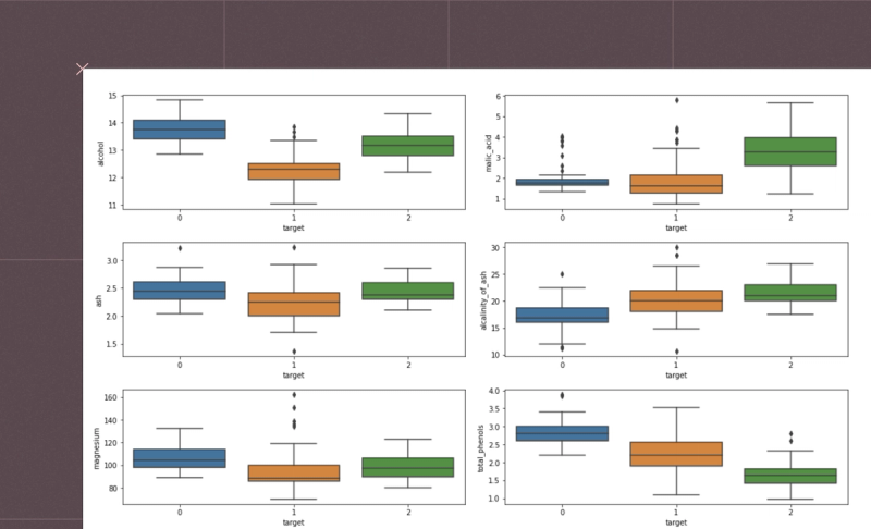
data.head(10)

This initial step loads data into our Python environment using Pandas. Here, the pd.read_csv() function is used to read a CSV (Comma-Separated Values) file from the URL. This CSV file, named wine_data.csv, contains our data related to wine: alcohol content, phenols, color.

Of course, we may not know that until we inspect the data. data.head(10) is where the initial inspection of the dataset occurs. The .head() method is a quick and efficient way to glance at the first few entries of the DataFrame; in this case, the first 10 rows. This initial peek is crucial as it provides insights into the structure of the data, including the column names (which indicate what each feature represents), the type of data in each column, and the format of the dataset.

For analysts and data scientists, this can inform how they might proceed with cleaning, processing, and analyzing the data. In the context of the wine_data.csv dataset, this could mean starting to form hypotheses about the relationships between different wine characteristics or planning preprocessing steps to make the data suitable for in-depth analysis or model building.

Preprocessing

Preprocessing is about cleaning our data and getting it into a format that can be passed to our models. Handling missing values is crucial for accurate results. data.isnull().sum() is used for this purpose:

data.isnull().sum()

It operates on a DataFrame data, where isnull() identifies missing values (NaNs or None) in each element, returning a Boolean DataFrame. The sum() method then counts these missing values in each column.

This concise operation provides a quick overview of missing data across columns, essential for data cleaning and preprocessing.

Then we standardize our data:

scaler = StandardScaler()
data = pd.DataFrame(data = scaler.fit_transform(data), columns = data.columns)

The StandardScaler is a tool from the scikit-learn library used for standardizing features by removing the mean and scaling to unit variance. Essentially, this process transforms each feature in the data to have a mean of zero and a standard deviation of one.

The next line, data = pd.DataFrame(data = scaler.fit_transform(data), columns = data.columns), applies this scaling transformation to the data DataFrame. The fit_transform method of the scaler standardizes the data and then returns it as a transformed NumPy array. This array is then converted back into a Pandas DataFrame with the same column names as the original data.

This step ensures that the scaled data retains its original structure and variable names, which is vital for interpretability in subsequent analysis. By standardizing the features, the data is normalized, reducing potential biases related to the scale of different features and making the dataset more suitable for applying machine learning algorithms.

Dimensionality Reduction

The core of this code is dimensionality reduction. We want to reduce the dimensions (features, or columns) we have on our dataset down into the ones that are critical for understanding the relationships within the dataset. Here, we’re going to use the modules from scikit-learn:

pca3D = PCA(n_components=3)
pca2D = PCA(n_components=2)

ica3D = FastICA(n_components = 3)
ica2D = FastICA(n_components = 2)

svd3D = TruncatedSVD(n_components = 3)
svd2D = TruncatedSVD(n_components = 2)

reduced3D = pd.DataFrame(data =  pca3D.fit_transform(data), columns = ['component_1', 'component_2', 'component_3'])
reduced2D = pd.DataFrame(data =  pca2D.fit_transform(data), columns = ['component_1', 'component_2'])

icareduced3D = pd.DataFrame(data =  ica3D.fit_transform(data), columns = ['component_1', 'component_2', 'component_3'])
icareduced2D = pd.DataFrame(data =  ica2D.fit_transform(data), columns = ['component_1', 'component_2'])

svdreduced3D = pd.DataFrame(data =  svd3D.fit_transform(data), columns = ['component_1', 'component_2', 'component_3'])
svdreduced2D = pd.DataFrame(data =  svd2D.fit_transform(data), columns = ['component_1', 'component_2'])

The code initializes PCA, ICA, and Truncated SVD for both 3D and 2D reduction. For instance, pca3D = PCA(n_components=3) and pca2D = PCA(n_components=2) create PCA objects tasked with reducing the data to three and two dimensions, respectively. Similar statements are used for ICA and Truncated SVD. These methods work by identifying and keeping only the most significant components (or features) of the data.

• PCA looks for directions that maximize variance

• ICA seeks statistically independent components

• Truncated SVD focuses on singular value decomposition, particularly useful for sparse datasets.

We then apply these techniques to the dataset using the fit_transform method. This method fits the model to the data and then transforms it into a lower-dimensional space. The transformed data is then framed into Pandas DataFrames with appropriate column names indicating the components. For instance, reduced3D holds the three-dimensional representation of the original data as transformed by PCA.

This is the core practice of dimensionality reduction enabling the visualization of complex data structures, enhancing computational efficiency, and revealing hidden patterns in the data that are not discernible in higher dimensions.

Clustering

With our data in a lower-dimension space, we can then cluster it ready for visualization and further analysis if needed. Clustering algorithms play a pivotal role in discovering underlying patterns in data. Here, we use the K-means clustering algorithm, a popular method used for grouping data into distinct clusters based on similarity.

kmeans = KMeans(n_clusters = 3)
reduced2D['cluster'] = kmeans.fit_predict(reduced2D)
icareduced2D['cluster'] = kmeans.fit_predict(icareduced2D)
svdreduced2D['cluster'] = kmeans.fit_predict(svdreduced2D)

pca_clusters3D = kmeans.fit_predict(reduced3D)
ica_clusters3D = kmeans.fit_predict(icareduced3D)
svd_clusters3D = kmeans.fit_predict(svdreduced3D)

We initialize the K-means algorithm, where kmeans = KMeans(n_clusters = 3) sets up a K-means model to identify three clusters within the data. The essence of K-means is to partition the data into clusters such that the sum of the squared distances between the data points and their respective cluster centroids is minimized.

Following the model initialization, the fit_predict method is applied to various reduced datasets. For instance, reduced2D['cluster'] = kmeans.fit_predict(reduced2D) assigns each data point in the 2D PCA-reduced dataset (reduced2D) to one of the three clusters. This process is repeated for datasets reduced by ICA and Truncated SVD in both 2D and 3D forms. The fit_predict method effectively performs two tasks: it fits the K-means model to the data and then assigns a cluster label to each data point.

The addition of the 'cluster' column to each DataFrame stores these labels, thereby categorizing each data point into a specific group based on its features.

Plotting

def plot_3D(components, cluster, title):
    if components.shape[1] != 3:
        raise ValueError(f"Components must be 3 dimensional. The components given have a dimensionality of {components.shape[1]}")
    
    frame = components.copy()
    x, y, z = frame['component_1'], frame['component_2'], frame['component_3']
    fig = px.scatter_3d(frame, x = 'component_1', y = 'component_2', z = 'component_3', color = cluster, title = title)
    # tight layout
    fig.update_layout(margin=dict(l=0, r=0, b=0, t=0))
    fig.show()

The plot_3D function is designed to create three-dimensional scatter plots. It takes three parameters: components, which is a DataFrame containing the data points to be plotted; cluster, which represents the cluster assignments of each data point; and title, a string that will be the title of the plot.

The function starts by ensuring that the components DataFrame has exactly three columns. This check is crucial because a 3D scatter plot, as the name suggests, requires exactly three dimensions to plot each data point in space. If the DataFrame does not have three columns, the function raises a ValueError, preventing any further execution and alerting the user to the issue.

After passing this check, the function proceeds to prepare the data for plotting. It first creates a copy of the components DataFrame to avoid altering the original data. Then, it extracts the individual components (presumably the x, y, and z coordinates for the 3D plot) from the DataFrame.

The core of the function uses Plotly Express, a plotting library known for its interactivity and aesthetically pleasing plots. The px.scatter_3d method is called to create a 3D scatter plot, with x, y, and z axes corresponding to the three components. The color of each data point is determined by the cluster parameter, allowing for easy visualization of how data points are grouped in clusters.

Finally, the function updates the layout of the plot to have a tight layout by setting the margins to zero, and then displays the plot with fig.show().

This 3D visualization can be particularly insightful, as it allows analysts to observe patterns and relationships in the data that might not be apparent in lower dimensions. For instance, in a dataset reduced to three principal components, such a plot can vividly illustrate how the data points are distributed across these principal components and how they are grouped into clusters.

We can then call this function for each of our dimensionality reduction techniques

plot_3D(reduced3D, pca_clusters3D, title = 'PCA in 3D')

plot_3D(icareduced3D, ica_clusters3D, "ICA in 3D")

plot_3D(svdreduced3D, svd_clusters3D, "")

In not a lot of lines of code, we’ve gone from a complex dataset that would be difficult to analyze with all features, to extracting just the most important features and being able to visualize the clustering of information. This demonstrates the power of dimensionality reduction techniques in simplifying data analysis, enabling us to uncover hidden patterns and insights that were not discernible in the original high-dimensional space.

These data analysis techniques underscore how crucial it is to effectively manage and interpret large datasets. By employing methods like PCA, ICA, and Truncated SVD for dimensionality reduction, we've managed to distill vast amounts of data into more manageable forms without losing critical information. Furthermore, the use of clustering algorithms like K-means has allowed us to identify natural groupings within the data, revealing underlying structures. The final step of visualizing these results, especially in 3D space, not only brings the data to life but also provides intuitive and tangible insights. This approach, balancing the depth of analysis with the clarity of visualization, is essential for making informed decisions in a data-driven world.