Blog
Getting started with linear regression
A common algorithm used to find the best-fitting line between two or more variables


Introduction to linear regression
Linear regression is a simple yet powerful predictive model aimed to learn the relationship between input variables and a target variable. To fully understand what it is and how it works, we're going to have to go back in time a bit.
Remember this equation from high school?
y = mx + b

This simple equation is used to draw a line on a grid. Let's break it down further to understand each of its terms.
- y: This is the dependent variable which tells us how far up or down the line is. This value depends on what happens on the right side of the equation.
- x: This is the independent variable which tells us how far along the line we are.
- m: This is the slope of the line which tells how steep the line actually is.
- b: This is the y-intercept which is the value of y when x is equal to 0.
What the Linear Regression algorithm does is try to learn the optimal values for m and b such that for any value of x we can accurately predict the value of y.
To understand this intuitively, say we want to be able to predict the price of a house based the area of the house 🏠 . The value we are trying to predict is house price and this prediction is dependent on the area of the house. If the area of the house is correlated with price, then as the house area increases we should also see an increase in price. This will allow us to learn the relationship between these two variables so that we can predict the price of a house for any area.
Now that we’ve gotten that out of the way, let’s see how we can implement this algorithm in Python.
We'll start by importing some useful libraries that we'll make use of later on.
import pandas as pd
import seaborn as sns
import numpy as np
from math import sqrt
import matplotlib.pyplot as plt
from sklearn.linear_model import LinearRegression
from sklearn.metrics import r2_score, mean_squared_error
from sklearn.model_selection import train_test_split
Dataset
Our dataset comes from Kaggle and contains information about the properties of a house as well as the price. You can download the dataset here.
df = pd.read_csv('Housing.csv')Data preprocessing
To keep it simple, we are only going to use the area of the house to predict the price. This means we must first create a subset of our original dataframe.
regression_data = df[['area', 'price']]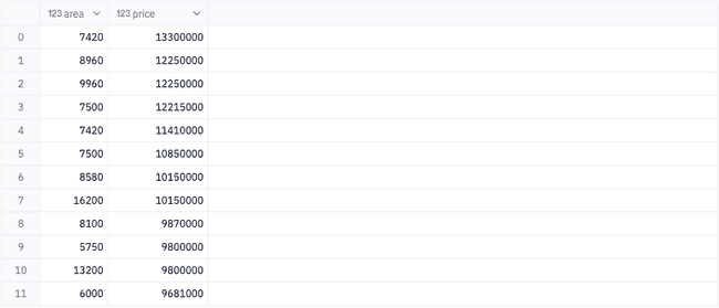
Let's create a scatter plot that can give us a quick visualization of the relationship between these two variables.
There seems to be an upward trend in our data, however, there also appears to be some minor clumping in the lower left corner of our scatter plot. This could indicate skewness in our data, so let's also visualize the distribution of each of our variables.
fig, (ax1, ax2) = plt.subplots(1, 2, figsize=(15, 5))
fig.suptitle('Distribution of price and area', size = 20)

# Create histograms for each variable
sns.histplot(ax = ax1, data = regression_data['area']);
sns.histplot(ax = ax2, data = regression_data['price']);

ax1.set_xlabel('area (Sq ft)');
ax2.set_xlabel('price ($1M)');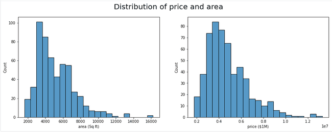
Just as expected, our data is right skewed. In most machine learning projects, skewness in your data is not ideal, but luckily there are ways to combat this. We will use a log transformation to shift our data towards a more normal distribution.
transformed = np.log(regression_data)

fig, (ax1, ax2) = plt.subplots(1, 2, figsize=(15, 5))
fig.suptitle('Distribution of price and area', size = 20)

# Create histograms for each variable
sns.histplot(ax = ax1, data = transformed['area']);
sns.histplot(ax = ax2, data = transformed['price']);

ax1.set_xlabel('Ln of area (Sq ft)');
ax2.set_xlabel('Ln of price ($1M)');
plt.show();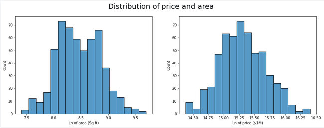
Now we can see a much more obvious trend in our data and the clumping from before is much less apparent.
Now that our data is symmetrical, we can split our data into a train and test set and begin training our model.
# convert the area pandas series into a numpy vector
inputs = np.array(transformed['area']).reshape(-1, 1)
target = transformed['price']
x_train, x_test, y_train, y_test = train_test_split(inputs, target, test_size=.2, random_state = 222)

model = LinearRegression()
model.fit(x_train, y_train)
Evaluation
Now that we have a trained regression model, we can inspect how well our model performs at predicting house prices. We first will call the predict() method on our test data set to obtain a set of predicted house prices.
predictions = model.predict(x_test)Keep in mind - these predictions are the log transformed values. In order to obtain a house price in dollars you will need to do the inverse of the original transformation using the np.exp function
Using our predicted values we can extract more metrics about our model's performance, like the r2 score and rmse, or root mean squared error.
- r2: Tells us how well our model fits to and explains our data. An r2 score of 1.0 means a perfect fit and our model can explain 100% of our dataset. An r2 of 0 means our model could not determine a predictable relationship in our dataset.
- rmse: Is the deviation of our prediction error. It tells us how far on average the data points are from the regression line. In other words it tells you how concentrated the data is around the line of best fit. For example, an rmse of 10 would mean that for whatever price we predict, we should expect the actual price to be within $10 of the predicted price.
rmse = round(sqrt(mean_squared_error(y_test, predictions)), 2)
r2 = round(r2_score(y_test, predictions), 2)
Lastly, we can extract the line of best fit, y = mx + b, by referencing the attributes model.coef and model.intercept_ from the model output to plot a regression line over our data.
slope = model.coef_[0]
intercept = model.intercept_
A slope of .51 means that every change in area by 1 unit translates to a .51 unit change in price. So if the price is $15.5 and the area is 8 sq ft, when the area increases to 9 sq ft, the price will be $16.
x = np.linspace(7, 10, 5)
y = [(slope * val) + intercept for val in x]
var = {'x': x, 'y': y}
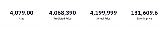
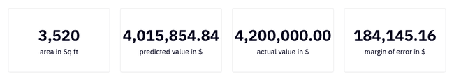
line = pd.DataFrame.from_records(var)Here we can further understand how well our model performed by actually seeing a predicted value vs actual values and the margin of error between them.
Multiple linear regression
In a simple linear regression model (which is what we just did), you are only using a single input value to predict your target. This simplicity makes it easy to visualize the data as well as understand how to implement the model. However, the results of a simple linear regression may not be the most accurate. One technique we can try to improve the accuracy of our model is to train a multiple linear regression model instead. The only difference being that this model can utilize multiple inputs to predict a target variable, hence the name.
For this, we will go back to our original dataset as input to our model.
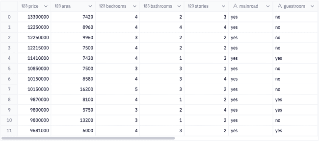
Encoding categorical variables
When working with most machine learning models, you will want your inputs to be a numerical value. The mathematical nature of these models makes columns like bedrooms = 4 or bathrooms = 2 to be easily understood. However, categories such as basement = Yes or furnish_status = furnished means nothing to the the model. What we need is a way to encode these categorical values so that the model knows how to give these values meaning. In this section of the tutorial we will look at how to one-hot encode our categorical values.
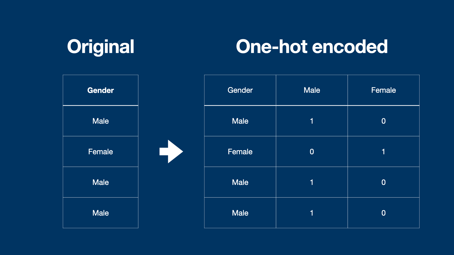
So what is one-hot encoding? Imagine I have a column in my dataset with two categories, say category1 and category2. If I want to show whether or not one of these categories is present for a given row, I can create new columns for each category and mark the row with a 1 if the category is present or a 0 if it is absent.
This essentially creates a binary list for each category in my column, which is more meaningful to the model than the category itself.
First, let's create a subset of our dataframe with only the categorical columns.
categorical_cols = [col for col in df.columns if df[col].dtype == 'object']
cats = df[categorical_cols]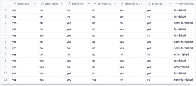
Luckily for us, a lot of these categorical variables are already essentially in binary. All we need to do is convert yes -> 1 and no -> 0, and we'll do this for all columns except furnishingstatus.
# replace yes with True and no with False
columns_excluding_furnishing = categorical_cols[:-1]
binary = cats[columns_excluding_furnishing].apply(lambda row: np.where(row == 'yes', 1, 0))
Next, we can use the function pd.get_dummies to one-hot encode furnishingstatus, and then combine the one-hot encoded dataframe with the binary dataframe.
oneHot = pd.get_dummies(cats['furnishingstatus'])
encoded = pd.concat([binary, oneHot], axis = 1)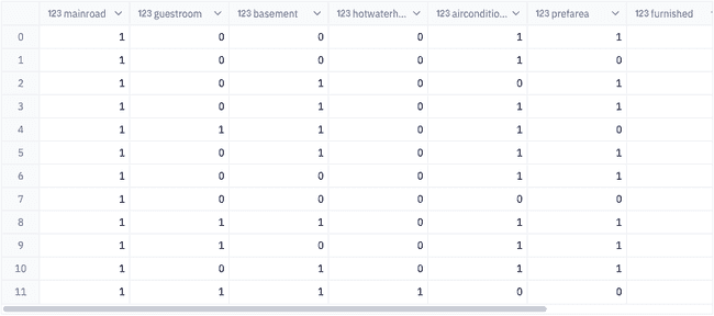
Lastly, let's remove our original categorical columns from our dataset to obtain a dataframe with numerical values only. Then we can combine this with our encoded dataframe.
# drop categorical columns from the dataframe
numerical = df.drop(columns = categorical_cols, axis = 1)

# recombine encoded columns with numerical features
data = pd.concat([numerical, encoded], axis = 1)

# transform price and area values to the log scale
data[['area', 'price']] = np.log(data[['area', 'price']])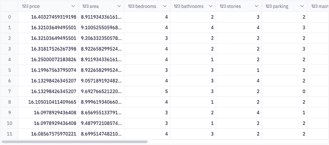
Now, we can start training our model.
inputs = data[data.columns[1:]]
target = data['price']
mul_x_train, mul_x_test, mul_y_train, mul_y_test = train_test_split(inputs, target, test_size=.2, random_state = 222)

model = LinearRegression()
model.fit(mul_x_train, mul_y_train)

y_pred = model.predict(mul_x_test)

multiple_mse = round(sqrt(mean_squared_error(mul_y_test, y_pred)), 2)
multiple_r2 = round(r2_score(mul_y_test, y_pred), 2)
Model comparison
In terms of best fit, the simple model has an r2 score of 34.0% and the multiple regression model has an r2 score of 72.0%. That's a 211.8% increase in performance!
In terms of error margin, the simple model has a rmse score of 0.33 and the multiple regression model has an rmse of 0.22. That's a 66.67% decrease in the margin of error!
Ideally, we want a model with a high r2 and a low rmse. This means that our multiple regression model would be the better model to use as it would give use accurate predictions that are more precise.
Here we can further understand how well our model performed by actually seeing a predicted value vs actual values and the margin of error between them.
Conclusion
Congratulations! You've successfully made it to the end of this tutorial 🤝.
Although simple, this tutorial introduced you to many concepts that are used in real machine learning tasks today. You learned how to perform data transformations, split data into train and test sets, fit a linear regression model, and evaluate its performance. There are also lots of things we didn't cover that we'll get to in future tutorials, so stay tuned and you will soon be a machine learning expert!!!
Related resources
If this is is interesting, click below to get started, or to check out opportunities to join our team.