Understanding the Importance of Stationarity in Time Series

“The Times They Are A-Changin” sang Bob Dylan in his famous ode to non-stationarity in time series.

Non-stationarity is a huge problem when you are analyzing time series. You don’t want the times to be a-changin’. If you’re trying to identify trends and use statistical models on time series, you want the opposite — stationarity. Stationarity refers to a dataset where the fundamental statistical characteristics of a time series — mean, variance, and autocorrelation — remain unwavering over time. This stability is not just an academic interest. It's the bedrock that permits you to do exploratory data analysis or apply robust statistical models to decipher and predict time series data.

So, how can you identify stationarity in any time series? That’s what we want to cover here: the main methods for decomposing your time series data and understanding the underlying trends and stationarity.

Stationarity in Time Series

Stationarity signifies that the statistical properties of time series, such as mean, variance, and covariance, remain constant over time, which is the fundamental assumption for many time series modeling techniques. It simplifies the complex dynamics within the data, making it more amenable to analysis, modeling, and forecasting.

There are two main types of Stationarity present in time series data.

Strict Stationarity

A time series is said to have Strict Stationarity if the joint distribution of its values at any set of time points is the same as the joint probability distribution of its values at any other set of time points. In simpler terms, the statistical properties of the data should not change at different time intervals. For example, if you are analyzing stock prices daily data, then according to strict stationarity, the statistical properties like mean and variance should remain constant across different days and years. Strict Stationarity is a strong assumption, and may not be satisfied by many real-world time series data.

Weak Stationarity

A time series is said to have Weak Stationarity if the mean and variance of the data remain constant over time, and the covariance between any two data points is a function of their time lag. It’s a more practical condition, as it allows for minor fluctuations in the data while preserving the essential statistical properties. Many real-world time series data can be approximated as weakly stationarity, making it a widely used assumption in time series analysis. This is also known as second-order stationarity or covariance stationarity.

Key Properties of Stationary Time Series

Several key properties come into play in stationary time series, setting it apart from its non-stationary counterparts. These properties serve as essential assumptions for many time series modeling techniques.

• Constant Mean: This is a fundamental property that states that the average value of the data remains consistent over time. In a stationary series, the mean does not exhibit any significant trend or fluctuation, making it a crucial characteristic for reliable analysis and modeling.

• Constant Variance: Another vital property is constant variance, which implies that the dispersion of data points remains constant over time. The absence of drastic changes in variance ensures that the data behaves predictably, allowing for better model accuracy.

• Auto-covariance Function: Auto-covariance measures the relationship between data points at different time lags. In a stationary time series, this function exhibits a consistent pattern. It reflects how correlated data points are with each other over time and plays a pivotal role in understanding the time series structure.

• Independence of Observation: In stationary time series, always remember that each observation is independent of the others. This means the value of a data point at one time does not depend on the value of the data point at any other time.

• Time-invariance: A stationary time series is time-invariant, meaning that the statistical properties of the data do not change with shifts in time. This ensures that the patterns and relationships within the data remain constant

• No Trend or Seasonality: Stationary time series typically lack significant trends or seasonality. Trend refers to a long-term upward or downward movement in the data, while seasonality involves repeating patterns at fixed intervals. The absence of these patterns in stationary data simplifies modeling and prediction tasks.

Why is Stationarity Crucial in Time Series Analysis?

Stationarity is really the foundational concept in time series analysis, so its importance cannot be overstated. This section explores the reasons why maintaining stationarity is so critical.

• Assumptions of many time series models. Stationarity is a fundamental assumption for numerous time series models such as ARIMA (Auto Regression Integrated Moving Average) and SARIMA (Seasonal ARIMA). These models rely on the constancy of statistical properties like mean and variance over time. Non-stationary data can lead to unreliable model outputs and inaccurate predictions, just because the models aren’t expecting it.

• Easier modeling and forecasting. Stationarity simplifies the complexities within time series data, making it easier to model and forecast than non-stationary time series. When the statistical properties of a time series remain constant over time, it’s much easier to use historical data to develop accurate models of the time series and forecast future values of the series.

• Interpretability of trends and patterns. Trends and patterns in stationary time series are easier to interpret because relationships between data points remain constant, which means that we can be confident that any trends or patterns we observe are not simply due to random fluctuations in the data.

• Enhanced diagnostic checks. Stationarity enables more robust diagnostic checks in time series analysis. By confirming stationarity, analysts can identify any potential issues in the data that might violate this essential assumption.

• Improved model performance. A stationary time series typically results in improved model performance. The constancy of key statistical properties ensures that models can better capture the underlying dynamics, leading to more accurate predictions.

Testing for Stationarity

Let’s explore the common statistical tests for stationarity. For this section, we will use the most popular Air Passengers Dataset, a commonly used time series dataset.

You can find this full analysis in a Hex notebook here.

Let’s first install all the necessary dependencies that we will use in this section.

$ pip install pandas numpy seaborn matplotlib statsmodels

# or

$ conda install pandas numpy seaborn matplotlib statsmodels

Once installed, we will import all the dependencies we are going to need:

# load dependencies
import pandas as pd
import seaborn as sns
import numpy as np
import matplotlib.pyplot as plt
from statsmodels.tsa.stattools import adfuller
from statsmodels.tsa.stattools import kpss
from statsmodels.tsa.seasonal import seasonal_decompose
from statsmodels.graphics.tsaplots import plot_acf, plot_pacf

# load the "Air Passengers" dataset from Seaborn
data = sns.load_dataset('flights')
data.head()

In the above code, the load_dataset() method from seaborn allows you to load the dataset. Now, let’s check the methods for detecting stationarity in time series data.

Common Statistical Tests for Stationarity

Augmented Dickey-Fuller (ADF) Test

The ADF test is a Hypothesis test used to assess whether a time series is stationary or not. The Null Hypothesis (H0) of the ADF test is that the time series is non-stationary, meaning it has a unit root. If the test statistic is less than the critical values, we reject the null hypothesis and conclude that the series is stationary.

The ADF tests calculate a test statistic, and the p-value associated with this statistic measures the strength of evidence against the null hypothesis. If the p-value is less than a chosen significance level (commonly set at 0.05), you reject the null hypothesis in favor of the alternative hypothesis concluding the time series as stationary.

# extract the number of passengers as a time series
passengers = data['passengers']

# perform the Augmented Dickey-Fuller (ADF) test
adf_result = adfuller(passengers)

# extract and print the test statistic and p-value
test_statistic, p_value, _, _, _, _ = adf_result
print(f'Test Statistic: {test_statistic}')
print(f'P-value: {p_value}')

# interpret the results
if p_value <= 0.05:
	print('Reject the null hypothesis: The time series is stationary.')
else:
	print('Fail to reject the null hypothesis: The time series is non-stationary.')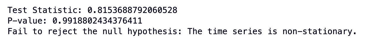

In the above code, we have used the adfuller() method from the statsmodels library and passed the passengers column values to it. The function returns the test_statistic, p_value which is crucial in identifying the presence of stationarity in time series data.

Kwiatkowski-Phillips-Schmidt-Shin (KPSS) Test

The KPSS test is another hypothesis test used to check for stationarity in a time series. The null hypothesis (H0) of the KPSS test is that the time series is stationary around a deterministic trend. If the test statistic is less than the critical values, we fail to reject the null hypothesis, indicating stationarity.

The KPSS test generates a test statistic and a p-value. In this test, if the p-value is greater than the chosen significance level (usually set at 0.05), you fail to reject the null hypothesis, indicating stationarity.

# perform the Kwiatkowski-Phillips-Schmidt-Shin (KPSS) test
kpss_result = kpss(passengers, regression='c')

print("\\nKPSS Test:")
print(f'Test Statistic: {kpss_result[0]}')
print(f'P-value: {kpss_result[1]}')

if kpss_result[1] > 0.05:
	print('Fail to reject the null hypothesis: The time series is stationary.')
else:
	print('Reject the null hypothesis: The time series is non-stationary.')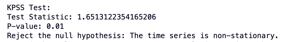

In the above code, we have used the kpss() method from the statsmodels library of Python to calculate the KPSS test. Simple!

Visual Methods for Detecting Stationarity

Visual methods for detecting stationarity offer a more intuitive approach to asses time series data. These methods are used to get a preliminary idea of stationarity in data.

Time Series Plots

A time series plot is a graph of time series data, with time on a horizontal axis and the values of the time series on the vertical axis. They display the data points over time, making it easier to observe trends, seasonality, and potential non-stationarity. There are different time series plots some of which are covered in this article.

Line Plot

A basic time series plot represents data points over time, making it easy to spot trends and patterns. The line plot visualizes the number of passengers over time, allowing you to identify trends. Below is a simple Python code to create a line plot for the Air Passengers dataset.

# create a line plot
plt.figure(figsize=(12, 6))
sns.lineplot(x=data.index, y=passengers)
plt.title('Air Passengers Time Series')
plt.xlabel('Year')
plt.ylabel('Number of Passengers')
plt.show()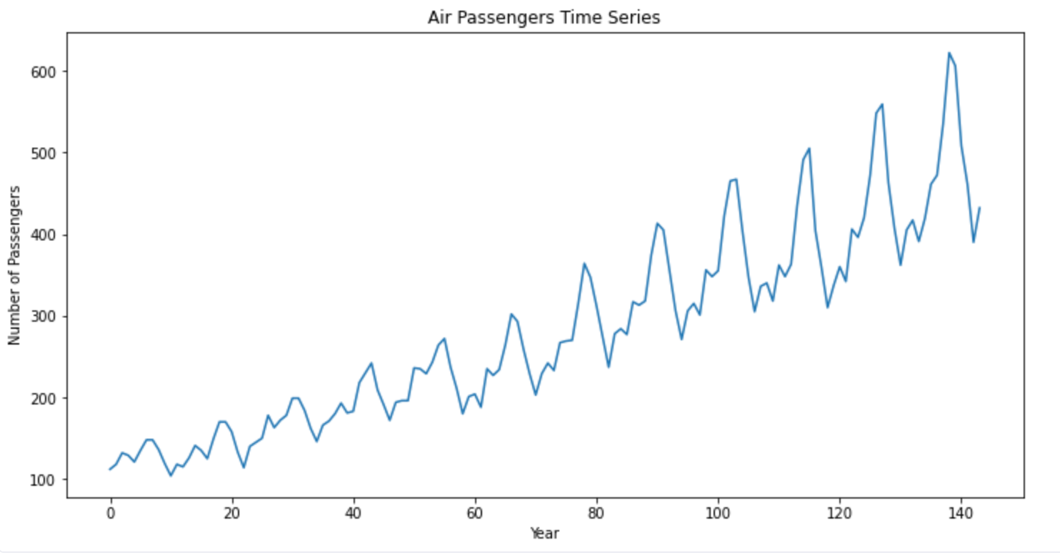

The lineplot() method from matplotlib helps you create the line plots. You can also add additional metadata such as labels, titles, colors, etc. to the plot to make them more appealing.

Seasonal Decomposition Plot

This plot decomposes a time series into its trend, seasonality, and residuals. It helps in understanding the underlying components of the data. Below is an example of creating a seasonal decomposition plot.

# make the datetime column as index
passengers.index = pd.date_range(start='1949-01', periods=len(passengers), freq='M')

# perform seasonal decomposition
decomposition = seasonal_decompose(passengers, model='additive')

# plot the decomposed components
decomposition.plot()
plt.show()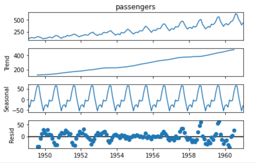

As you might have noticed, to create the seasonal decomposition graph, you need to make the datetime column the index. Then, using the seasonal_decompose() method from statsmodels, you can visualize different seasonal components of the time series.

In both the graphs mentioned above, you can observe that data has trends and seasonality but it is non-stationary.

ACF and PACF plots

Autocorrelation Function (ACF) and Partial Autocorrelation Function (PACF) plots are used to visualize the autocorrelation in time series data. The ACF plot shows the correlation between a time series and its lagged values at different time lags. It is useful for identifying seasonality and lag patterns. Here’s how to create an ACF plot.

# create an ACF plot
plot_acf(passengers, lags=50)
plt.title('Autocorrelation Function (ACF) Plot')
plt.show()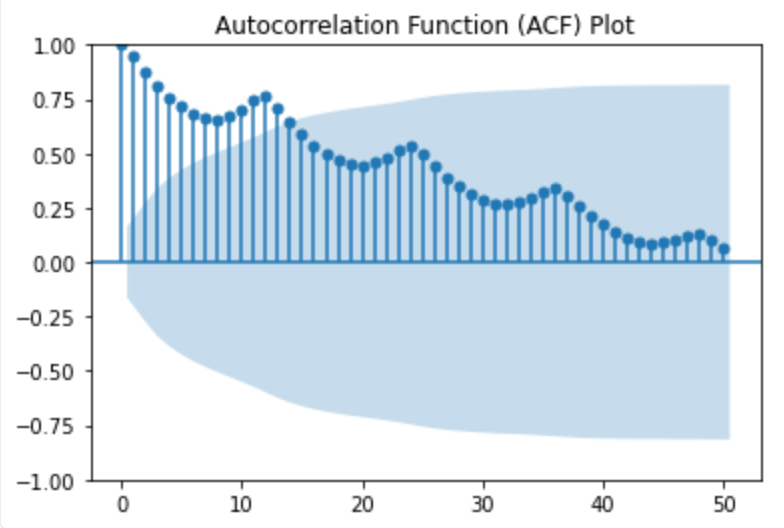

The PACF plot shows the partial correlation between a time series and its lagged values while controlling for the influence of shorter lags. It helps identify the order of the autoregressive (AR) term in ARIMA modeling. Here’s how to create a PACF plot. The PACF plot can assist in determining the order of the AR term in your time series model.

# create an PACF plot
plot_pacf(passengers, lags=50)
plt.title('Partial Autocorrelation Function (ACF) Plot')
plt.show()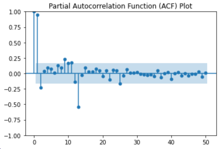

How to Interpret the Results of Stationarity Tests?

Interpreting the results of stationarity tests is crucial for making informed decisions about time series data. Here are key points to consider when interpreting the results.

• Look at the P-Value: The p-value is the probability of obtaining a test statistic as extreme as or more extreme than the observed test statistic under the null hypothesis. A small p-value indicates that the null hypothesis is unlikely to be true, and therefore the time series is stationary.

• Consider Multiple Tests: It’s often beneficial to perform both ADF and KPSS tests and interpret their results in combination. If one test suggests stationarity and the other suggests non-stationarity, carefully assess the specific characteristics of the data and any potential transformations.

• Compare the Test Statistics to the Critical Values: Critical values are provided in statistical tables for different significance levels. If the test statistic is less than the critical value, then the null hypothesis of a unit root is rejected, and the time series is concluded to be stationary.

• Context Matters: Consider the context of the data and the goals of your analysis. Some non-stationarity may be acceptable, depending on the problem. For example, financial data often exhibits trends and may still be suitable for modeling.

Non-Changin’ Times Make For Better Analysis

Obviously, we can’t all have Dylan’s implicit knowledge of time series and the dangers of change. But hopefully with this primer on testing for stationarity in your own datasets you’ll be a little closer to the Minnesota Bard.

Making this a core part of your exploratory data analysis when dealing with any time series data will help you perform better analysis and understand any results better. Performing these tests acts as a fork in the road, guiding your subsequent analytical strategy. If your tests indicate that your time series is stationary, then you can proceed confidently with models that assume stationarity. On the other hand, if your time series exhibits non-stationarity, you'll be steered towards techniques designed to stabilize your data, such as differencing or transformation, before embarking on further analysis.

Embracing stationarity testing is not only about ensuring the applicability of certain statistical methods; it's about comprehensively understanding the behavior and structure of your time series data. It prepares you to mitigate potential pitfalls and capitalize on the insights that only well-conditioned time series data can offer.