Build, test, and deploy powerful ML models

As data volume expands and computational capabilities increase, the demand for sophisticated models that can interpret complex datasets and deliver actionable insights is paramount. This shift has spotlighted the need for a robust methodology in model development. Analysts face the challenge of not only creating models that are accurate and efficient but also ensuring these models are scalable and reliable in diverse operational environments.

We want to show you how to develop these robust machine learning models and methodologies within Hex. Building with Hex will mean you can take advantage of popular ML libraries for analysis, pull data directly from your data warehouse, and share both the results and the code for your models with your team.

Understanding Machine Learning Model Development

Before jumping into machine learning, we must understand what goes into building a machine learning model.

1. Define the Problem

Defining the problem is the foundational step in machine learning model development. It involves understanding and articulating what you aim to solve with the machine learning model. This step requires a clear comprehension of the business or research objectives, the nature of the problem (such as classification, regression, clustering, etc.), and the solution's impact. A well-defined problem statement guides the entire machine learning process, ensuring that the developed model aligns with the desired outcomes.

2. Data Collection

Data collection is a critical phase of gathering relevant data to train the machine learning model. This step involves identifying the necessary data sources and ensuring the data is sufficient, relevant, and high-quality. Data can come from various sources, including internal databases, public datasets, or real-time data streams. The quantity and quality of collected data significantly influence the machine learning model's performance.

3. Preparing the Data

Preparing the data involves cleaning, transforming, and normalizing it to make it suitable for training a machine learning model. This step may include handling missing values, dealing with outliers, encoding categorical variables, and normalizing numerical values. Data preparation is crucial as it directly impacts the model's ability to learn effectively from the data.

4. Choosing a Model

Choosing a model involves selecting an appropriate machine learning algorithm based on the problem definition, data characteristics, and desired outcome. Different models, such as decision trees, neural networks, or support vector machines, have their strengths and weaknesses depending on the type and complexity of the problem. The choice of model can significantly affect the performance and accuracy of the final solution.

5. Training the Model

Training the model is the process where the chosen machine learning algorithm learns from the prepared data. During this phase, the model iteratively adjusts its parameters to minimize prediction errors. Training involves splitting the data into training and validation sets to ensure the model can generalize well to new, unseen data.

6. Evaluating the Model

Evaluating the model is a critical step to assess its performance. This step involves using various metrics like accuracy, precision, recall, or mean squared error, depending on the problem type. Evaluation is typically done using a separate test dataset the model has not seen during training, providing insights into how well the model will perform in real-world scenarios.

7. Parameter Tuning

Parameter tuning, or hyperparameter optimization, is the process of fine-tuning the model's settings to improve its performance. This step involves experimenting with different configurations of the model's hyperparameters, which are not learned from the data but set prior to the training process. Effective parameter tuning can significantly enhance a model's accuracy and efficiency.

8. Making Predictions

Making predictions is the final step, where the trained and tuned model is used to predict outcomes on new data. This is the stage where the model's practical value is realized as it applies its learned patterns to provide insights, make decisions, or automate tasks. The model's predictions can be used to drive business decisions, inform research, or power intelligent applications.

Machine Learning Model Development with Hex

We will develop a machine learning model for churn prediction. Churn refers to the rate at which the customers or subscribers stop using products or doing business with a company during a particular period. It is also popular with names customer attrition or customer turnover. A business needs to identify the churn rate as it is quite expensive to obtain new customers rather than satisfy existing ones.

We will develop a classifier ML model to use customer data and predict whether the customer will churn. This model will also be able to tell us what features play a key role in identifying what causes churn so that businesses can make informed decisions.

This section will use the Python 3.10 language and Hex as a development platform. Hex is an effective development environment for developing and implementing predictive models. It easily integrates different databases and warehouses to read and write data efficiently. We will install Python dependencies using the Python Package Manager (PIP). Also, we will use a feature in Hex called Component that allows you to reuse code in multiple projects from a single source of truth.

Install and Load Dependencies

Let’s start with installing the necessary dependencies.

$ pip install pandas numpy
$ pip install matplotlib seaborn
$ pip install scikit-learn
$ pip install imbalanced-learn

Once you have installed the necessary dependencies you can import them into the Hex environment as follows:

import pandas as pd
import numpy as np
import seaborn as sns
import matplotlib.pyplot as plt
import sklearn
from sklearn.model_selection import train_test_split
import sklearn.linear_model as linearModels
import sklearn.ensemble as ensembleModels
from sklearn.preprocessing import StandardScaler
from sklearn.metrics import confusion_matrix, accuracy_score, precision_score, recall_score, roc_auc_score, classification_report

Exploring the Data

The data that we are going to use is stored in the Snowflake warehouse. You can use the SQL command to load this data in the Hex environment. This data is loaded as a DataFrame so that it will become easy for you to apply various Pandas operations for data cleaning and preparation.

select * from "DEMO_DATA"."DEMOS"."TELECOM_CHURN"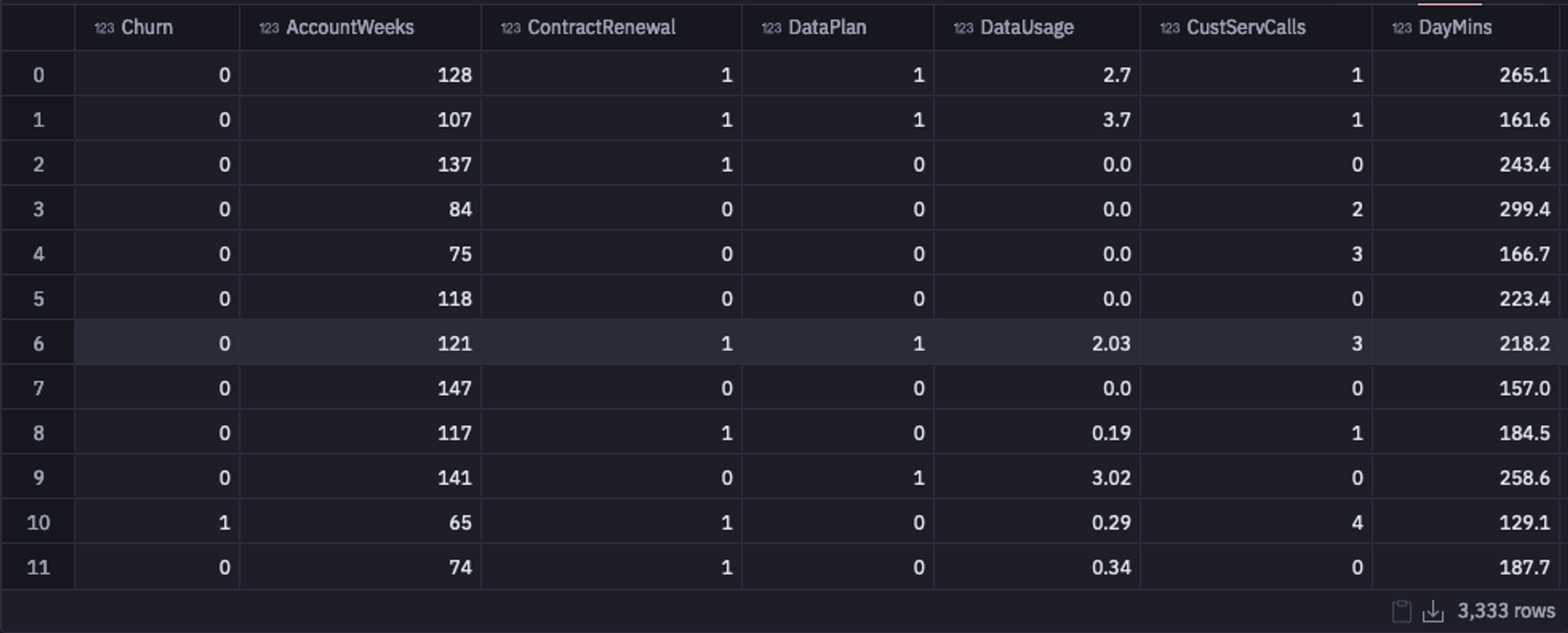

Select Data from Warehouse

The first thing that we are going to do is check the number of null values in all the features in our dataset.

data.isnull().sum()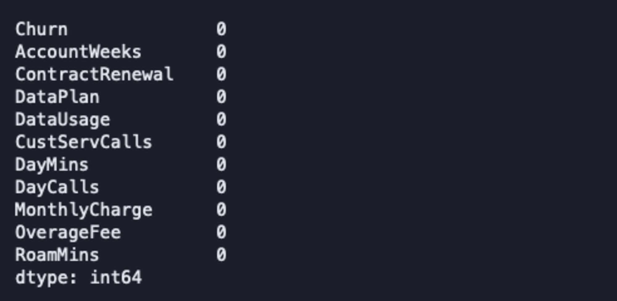

Check Null Values

As you can see, there are no NaN values in any of our features in the dataset. But if there were any, you can either drop them (not recommended due to information loss) or replace them with a measure of central tendency if they are missing at random.

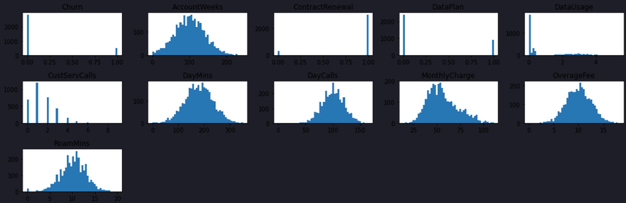
Next, let’s check the data distribution for all the features in the dataset by plotting the histograms as follows:

plt.figure(figsize=(15, 5))
for i, (k, v) in enumerate(data.items(), 1):
	plt.subplot(3, 5, i)  # create subplots
	plt.hist(v, bins = 50)
	plt.title(f'{k}')

plt.tight_layout()
plt.show();

Check Data Distribution

As you can see in the above graphs, most of these features follow the normal distribution so there is no need to do anything on this part.

Then let’s check the Correlation (Pearson) of each column with our target feature Churn to check the relationship among them. The correlation value 1 and -1 show a strong correlation while the value 0 represents no correlation between the features. You can calculate it using the corr() method and then you can easily visualize them using the heatmap.

mapping = data.corr().iloc[:, :1]
sns.set(rc={'figure.figsize':(2,5)})
sns.heatmap(mapping, annot = True);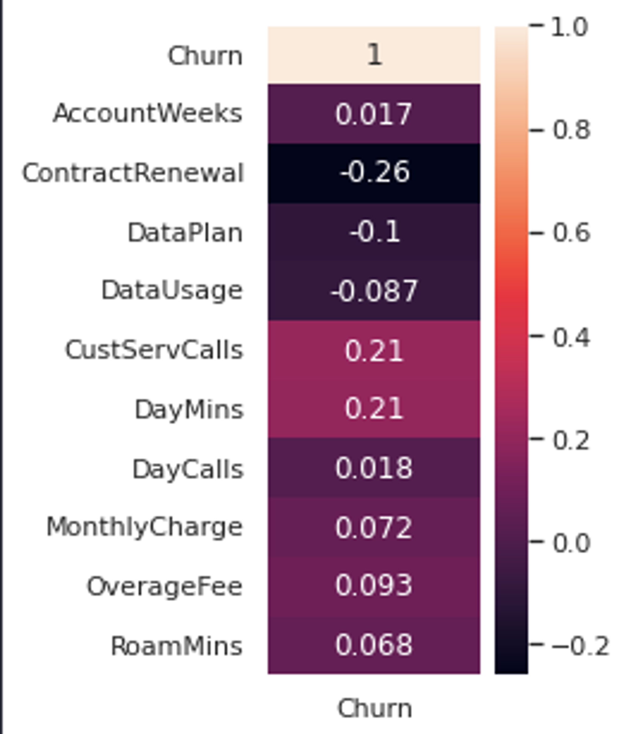

Check Correlation

As per the above image, features CustServCalls, DayMins, and ContractRenewal represent the strongest correlation which means these variables might be important for our model.

Note: Usually the highly dependent features (corr > 0.7) are dropped from the dataset as these features do not bring much information to a dataset but add a lot of complexity.

Finally, since we are working on the classification use case, we will check the output feature’s distribution to get an insight into what we are dealing with.

churn_ratios = data['Churn'].value_counts(normalize = True).values
pos = churn_ratios[0]
neg = churn_ratios[1]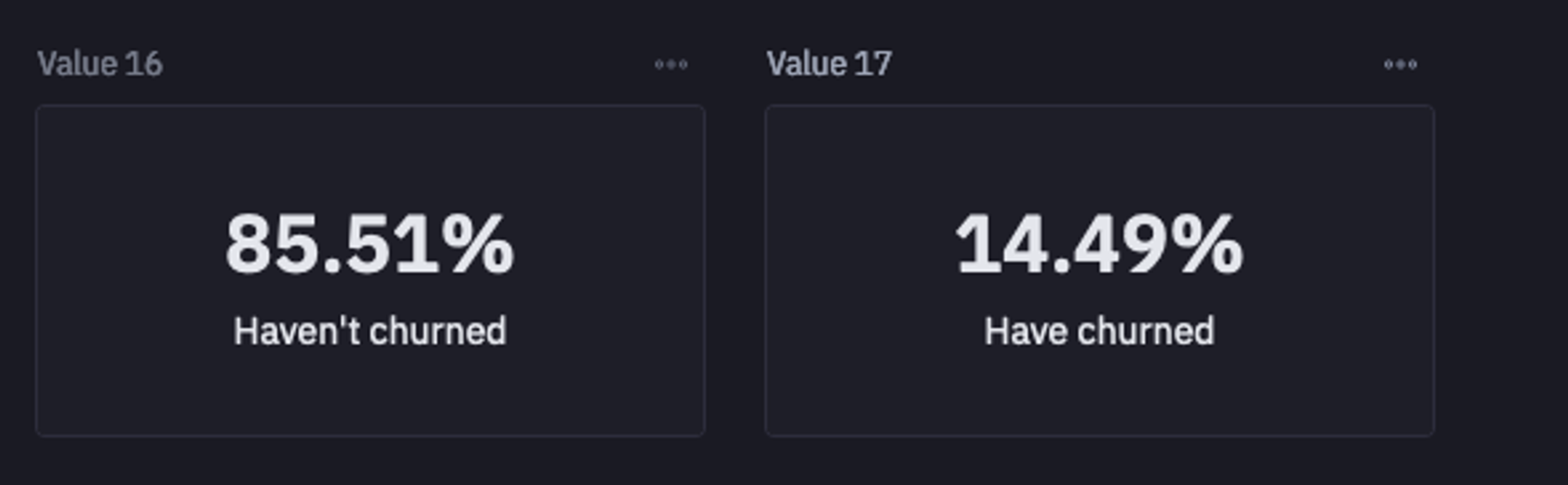

Output Class Distribution

As you can see, the data is highly imbalanced i.e. the number of customers that will churn (minority class) is way less than the number of customers that will not (majority class). This type of data is not ideal for a machine learning model as the model will pay more attention to the majority and will be highly biased toward those. As a result, the predictions made using the model will be biased toward the majority class and it will fail to predict the minority class. We will discuss the solution to this problem in the upcoming section.

You can also visualize the plot of class distribution in Hex, it will look something like this:

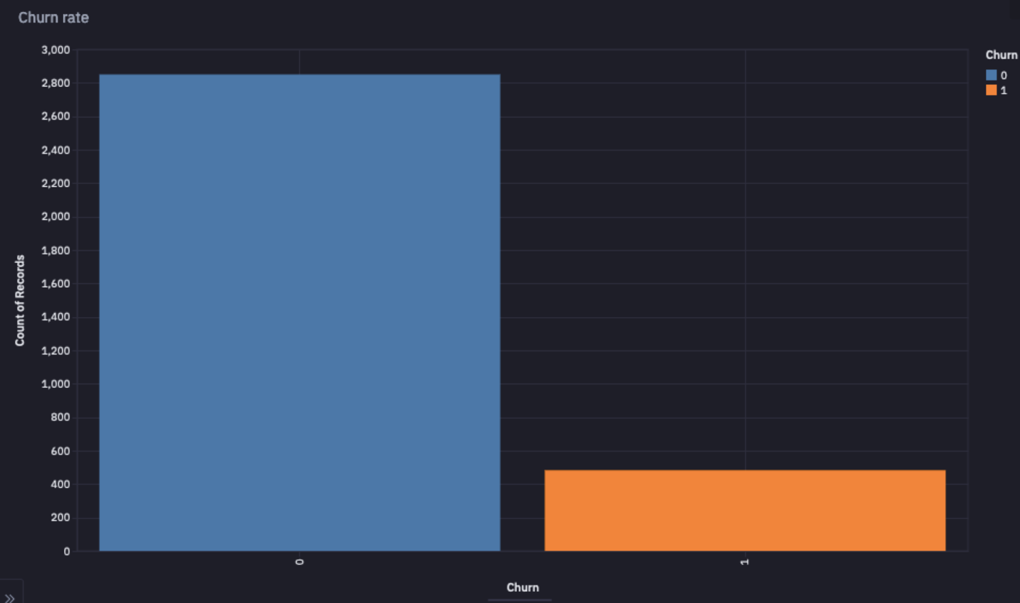
Output Class Distribution Plot

Modeling with Imbalanced Dataset

We will first train the ML model with the imbalanced dataset to have a look at how it affects the model performance.

total = sum(data['Churn'].value_counts())
majority = data['Churn'].value_counts().max()
imbalanced_baseline = majority / total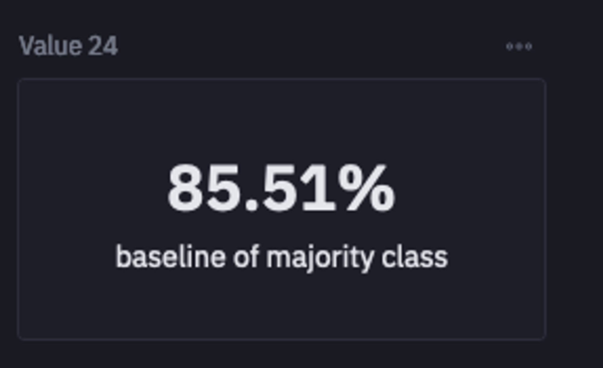

Non Churn Ratio

The 85% of our data is made up of non-churn cases.

The model that we are going to use for this tutorial is Random Forest Classifier which is an ensemble learning technique for classification. This algorithm works by creating multiple subsets of the original dataset and training different decision tree classifiers on these subsets of data. An average is taken for the results of these decision trees to improve the predictive accuracy of that dataset.

We will also scale all our features using the Standard Scaler so that values in each feature will be at the same scale and reduce the bias toward features with larger values.

# To scale our data
scaler = StandardScaler()

# Extract the training features
features = [col for col in data.columns if col != 'Churn']
features = data[features]

# extract the target
target = data['Churn'].to_numpy()

# Scale training features
scaled_features = scaler.fit_transform(features)

Then to test the predictive performance of our model on the unseen data, we will split the original data into training and testing sets using the train_test_split() method from sklearn.

# split into train set and test set
x_train, x_test, y_train, y_test = train_test_split(
	scaled_features, target, train_size=0.8, random_state=444
)

Finally, we will create an object of RandomForestClassifier() and will call the fit() method that accepts the input data and returns a trained model.

# Instantiate model
imbalanced_model = ensembleModels.RandomForestClassifier()

# train the model
imbalanced_model.fit(x_train, y_train)

Model Evaluation

Now that you have trained your ML model, it is time to check its performance on the unseen data (testing set). In ML, performance evaluation is done with the help of evaluation metrics. For classification models, the popularly used metrics are accuracy, precision, recall, F1-score, and AUC-ROC curve. For this model, we will be focusing on three metrics:

• Accuracy:

  Accuracy is the measure of number of correct predictions out of the total number of predictions.

• Precision:

  Precision tells us, out of all the positives that the model has predicted, how many of them are true.

• Recall:

  Recall tells us, out of all the positives in our dataset, how many of them the model has predicted as true.

Note: In the case of the imbalanced dataset, accuracy is not the right measure. For example, there are 90 negative samples and 10 positive samples in your testing set. If your model (trained on imbalanced data) has predicted all 100 samples as negative then your model accuracy would still be 90% but ideally, the model is not useful.

To check these metrics in Hex, you can use the following code:

# Used in single-value cells
imbalanced_predictions = imbalanced_model.predict(x_test)
imbalanced_accuracy = round(accuracy_score(y_test, imbalanced_predictions), 3)
imbalanced_precision = round(precision_score(y_test, imbalanced_predictions), 3)
imbalanced_recall = round(recall_score(y_test, imbalanced_predictions), 3)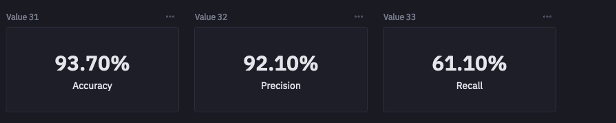

Model Evaluation

As you can see in the above image, the accuracy and precision of the models are quite good but the recall is a little less. Now the major question that you should be asking is, which one is more important for your use case? The choice of metrics really depends on the type of use case you are working on. For instance, in this churn use case, we care about the number of positives getting detected as true. If we predict some negatives as positives (false positives) there would not be any issue but if the model predicts positives as negatives (false negatives) or in simple terms predicts churn cases as not churn then it can surely harm business.

So clearly, recall is something that we need to focus on for churn analysis, and the model with an imbalanced dataset is not giving a good recall score.

Modeling with a Balanced Dataset

To improve the recall, we need to balance the number of minority and majority classes in the dataset. The popular method used for this is resampling which aims to create new samples or delete existing ones from the original dataset. There are two different ways to remove imbalance using resampling:

• Downsampling:

  Sometimes also referred to as undersampling, this method removes the samples from the majority class to bring them to the level of the minority class. This method is not always recommended as you can potentially lose some important information from dropping the samples. Some of the popular undersampling methods are

  Near Miss Undersampling, Tomek Links for Undersampling, One-Sided Selection for Undersampling, etc.

• Upsampling:

  Also referred to as oversampling, this method aims to increase the number of samples of minority classes to bring them to a level of majority classes to balance the dataset. Some of the popular upsampling methods are SMOTE, ADASYN, Borderline Oversampling, etc.

Note: You can also apply a combination of upsampling and downsampling methods together to suit the specific needs of your dataset.

For our churn dataset, we will use the SMOTE upsampling method. To do so, you can use the imblearn library which has an implementation of all sampling methods. Now let’s apply the SMOTE method to the dataset and train the RFC model again.

from imblearn.over_sampling import SMOTE

# Instantiate model
model = ensembleModels.RandomForestClassifier(random_state = 222)

# To scale our data
scaler = StandardScaler()

# Extract the training features
features_names = [col for col in data.columns if col != 'Churn']
features = data[features_names]

# Scale training features
scaled_features = scaler.fit_transform(features)

# extract the target
target = data['Churn'].to_numpy()

# upsample the minority class in the dataset
upsampler = SMOTE(random_state = 111)
r_features, r_target = upsampler.fit_resample(scaled_features, target)

# split into train set and test set
x_train, x_test, y_train, y_test = train_test_split(
	r_features, r_target, train_size=0.8, random_state=444
)

# Train the model
model.fit(x_train, y_train)

Train Model with Balanced Dataset

You can have a look at the number of samples from each class with the help of the following code:

total = sum(up['Churn'].value_counts())
majority = up['Churn'].value_counts().max()
baseline = majority / total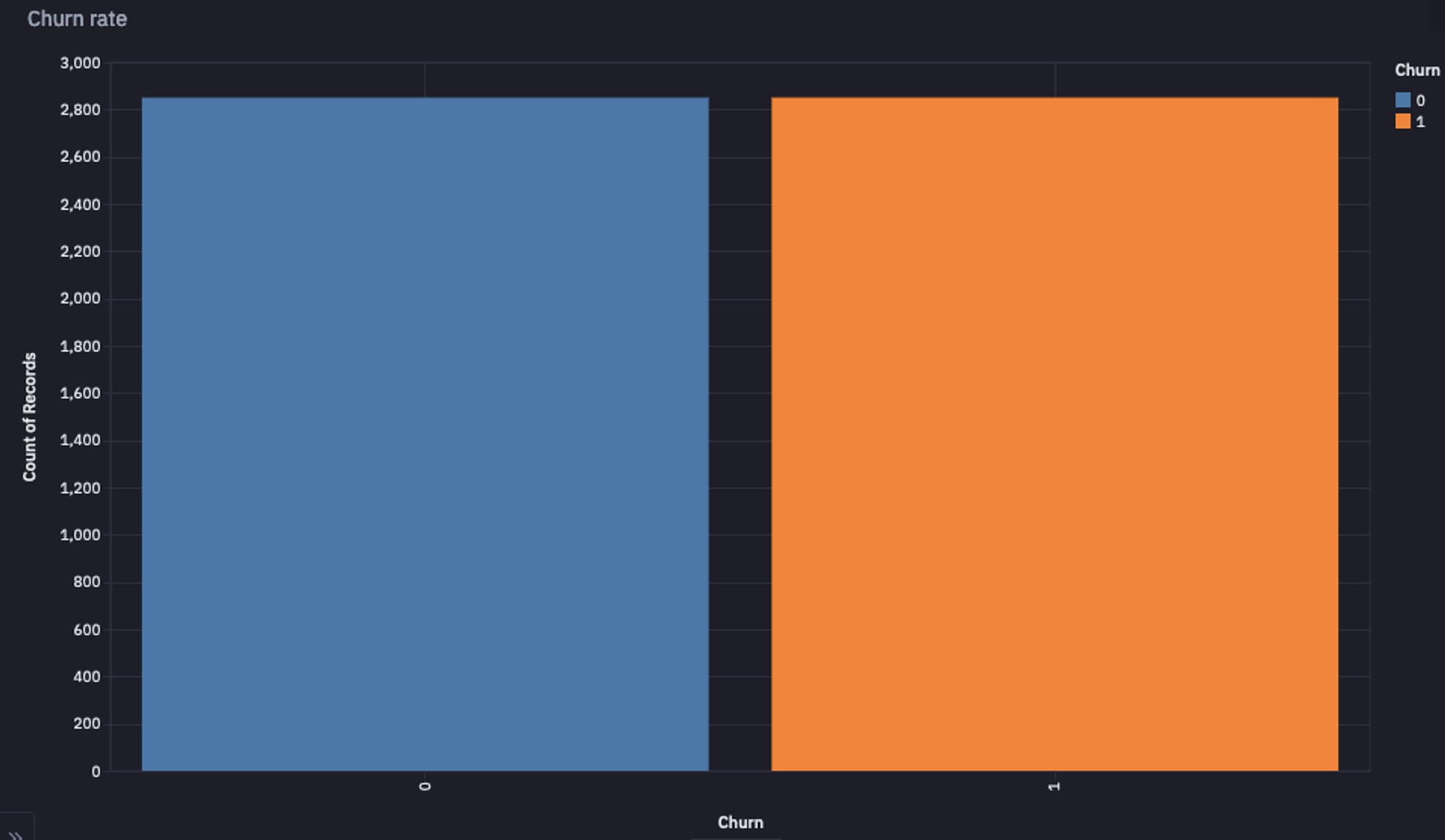

Resampled Data

Note: Ideally you should apply the sampling methods to the training dataset only so that the testing dataset will still have the real samples to test the actual model performance.

Metrics and Interpretation

Next, you can check the performance of this newly trained model on the balanced dataset:

accuracy = round(accuracy_score(y_test, predictions), 3)
precision = round(precision_score(y_test, predictions), 3)
recall = round(recall_score(y_test, predictions), 3)
auc_roc = round(roc_auc_score(y_test, predictions), 3)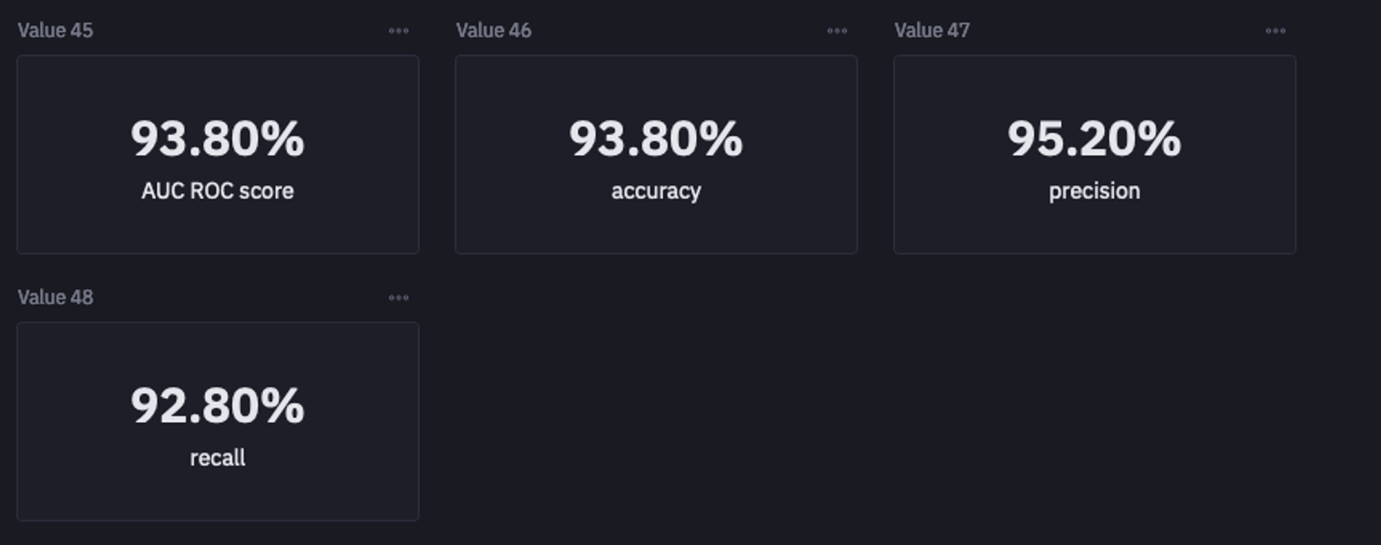

Model Performance on Balanced Dataset

As expected, the recall score has improved a lot along with the good accuracy, precision, and AUC-ROC score. As a result, our model is good enough to be used for determining the churn cases for the business.

There is one last thing that you need to perform before wrapping up the development of the ML model. In some cases, when the model is not performing well, it could be the case that some of the features are not contributing to the prediction. It is a good idea to check the feature importance (how important a feature is to the model) for the following reasons:

• Feature selection:

  It helps select the best features from the dataset that are actually contributing to the model’s performance. This results in reducing the number of features while keeping the performance of the model nearly the same.

• Feature Understanding:

  For some of the use cases such as churn, it is helpful to get the gist about what features are causing the churn so that the business can take action accordingly.

To check the feature’s importance, you can use the following chunk of code:

importances = pd.DataFrame(
	list(zip(features.columns, model.feature_importances_)),
	columns=["feature", "importance"],
)

bal = importances.sort_values(by = 'importance', ascending=False)['feature'].iloc[:5].to_list()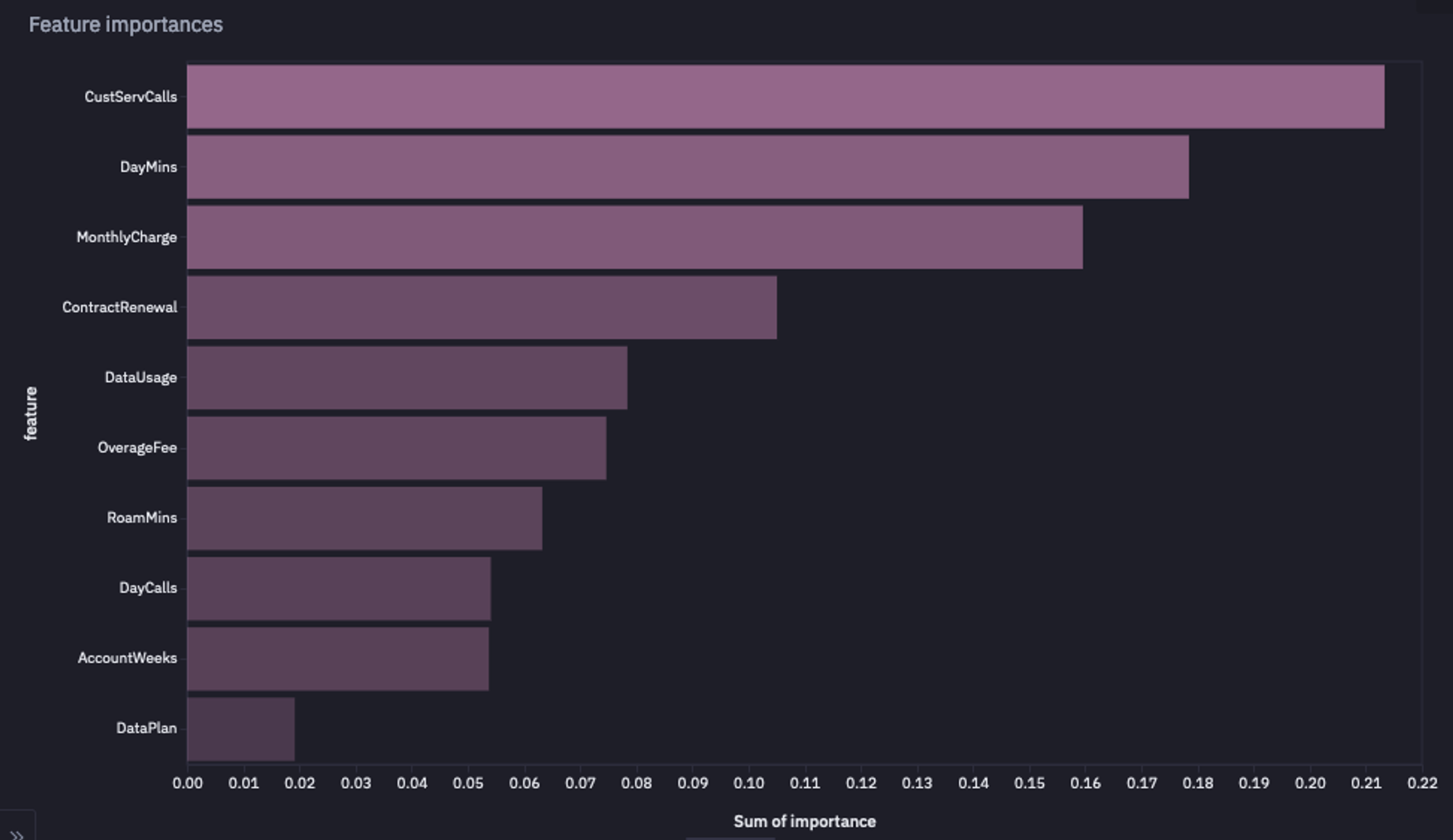

Feature Importance Graph

As you can see, CustServCalls, DayMins, and MonthlyCharge are the most important features for our churn analysis.

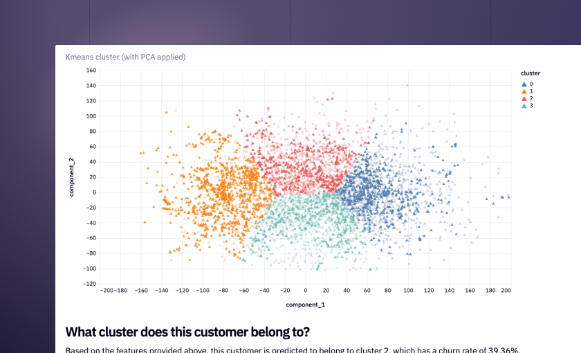
This is it, you have now developed your own churn prediction machine learning model using Python and Hex. If you would like to play around with this churn model, check out this interactive dashboard project.

This article gives you a starting point to develop your own ML models, you can apply this knowledge to other use cases to improve your understanding of concepts.