Scaling Hierarchical Clustering

One part of using clustering algorithms I’ve always found weird is that you have to specify the number of clusters you want in advance. If I knew that, I wouldn’t need an algorithm to help me, surely?

That makes hierarchical clustering stand out from its data clustering brethren—it works out the number of clusters you need. It goes a little further and gives you clusters of clusters, and clusters of clusters of clusters.

But you might be able to spot a flaw in that last sentence. Generally, anything that scales like that with groups of groups of groups doesn’t scale well. That’s the critical flaw with hierarchical clustering. Its computational complexity is cubically proportional to the dataset size, which is bad.

As datasets continue to grow in volume and dimensionality, these algorithms' computational and memory demands become untenable.

But datasets aren’t getting smaller anytime soon. The pressing need to analyze large datasets efficiently means people have been exploring mechanisms for scaling hierarchical clustering without substantially compromising the quality of results. Here, we’re going through a few of them in the hopes they can help you when using this method.

The Basics of Hierarchical Clustering

Let’s start with how hierarchical clustering works so we can begin to see what goes wrong.

Hierarchical clustering is a systematic approach in data science to building a hierarchy of clusters. The core objective is to create a tree of clusters, often visualized as a dendrogram, where each leaf node is a single data point, and the topmost node represents the entire dataset.

There are two types of hierarchical clustering: Agglomerative vs. Divisive.

Agglomerative clustering is a bottom-up approach. Initially, every data point is treated as a single cluster, and the algorithm proceeds by iteratively merging the closest pair of clusters. This process continues until there's just one cluster left, encompassing all data points.

Let’s show this quickly with the iris dataset:

from sklearn.datasets import load_iris
import matplotlib.pyplot as plt
import scipy.cluster.hierarchy as sch
import pandas as pd

# Load iris dataset
data = load_iris()
iris_df = pd.DataFrame(data.data, columns=data.feature_names)

# Compute the linkage matrix for hierarchical clustering
Z = sch.linkage(iris_df, method='ward')

# Plot the dendrogram
plt.figure(figsize=(10, 7))
dendrogram = sch.dendrogram(Z)
plt.title('Dendrogram')
plt.xlabel('Samples')
plt.ylabel('Euclidean distances')
plt.show()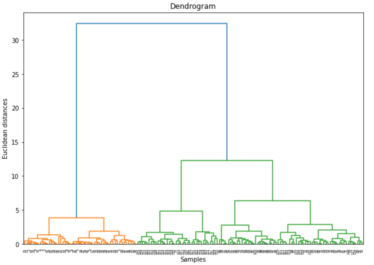

Divisive clustering is a top-down approach. It begins with the entire dataset treated as a single cluster. The algorithm then recursively splits the cluster into smaller clusters until each data point is in its own cluster. While more computationally intensive, this approach can occasionally yield better results for certain datasets.

Several distance metrics can be employed to compute the 'distance' between data points or clusters:

• Euclidean Distance: The straight-line distance between two points in Euclidean space.

• Manhattan Distance: The sum of absolute differences between coordinates, often relevant in grid-like structures.

• Cosine Similarity: A measure of cosine of the angle between two non-zero vectors, useful for high-dimensional data.

A dendrogram, a tree-like diagram, shows the arrangement of the clusters created by hierarchical clustering. Each merge or split is represented by a horizontal line. The vertical lines, on the other hand, represent clusters that were merged or split, with height denoting the level at which the merge or split happened.

Let’s show what this all looks like with the iris dataset:

from sklearn.datasets import load_iris
import matplotlib.pyplot as plt
import scipy.cluster.hierarchy as sch
import pandas as pd

# Load iris dataset
data = load_iris()
iris_df = pd.DataFrame(data.data, columns=data.feature_names)

# Compute the linkage matrix for hierarchical clustering
Z = sch.linkage(iris_df, method='ward')

# Plot the dendrogram
plt.figure(figsize=(10, 7))
dendrogram = sch.dendrogram(Z)
plt.title('Dendrogram')
plt.xlabel('Samples')
plt.ylabel('Euclidean distances')
plt.show()

Some nice clusters, and we haven’t had to give the algorithm any hints.

How Scaling Hierarchical Clustering Goes Wrong

The Iris dataset is small, so hierarchical clustering is a great option. But not all datasets are as manageable. The challenges in scaling this method predominantly stem from computational, memory, and quality perspectives.

Computational Complexity

The computational cost is a primary concern when it comes to hierarchical clustering. Basically, every point has to be assessed in position to every other point. This means that, as the number of points grows, these pairwise computations explode.

In the naive agglomerative clustering approach, the is a huge problem. During each of its iterations, the algorithm recalculates the distances between every pair of clusters to determine the closest ones to merge. This leads to a formidable time complexity of $O(n^3)$. This cubic growth rate is particularly problematic as datasets grow, making it a non-starter for large-scale data.

# Hypothetical representation of naive agglomerative approach
for i in range(n):
    for j in range(n):
        for k in range(n):
            if some_condition(i, j, k):
                distance_matrix[i][j] = compute_distance(data[i], data[j])

Thankfully, there are more sophisticated methods that leverage advanced data structures (like priority queues) and algorithmic strategies (like divide-and-conquer). These refined techniques can reduce the time complexity to $O(n^2 \log n)$. While this is a significant improvement, it's still quadratic in nature, which means it can struggle with very large datasets. This is how this looks when visualized:

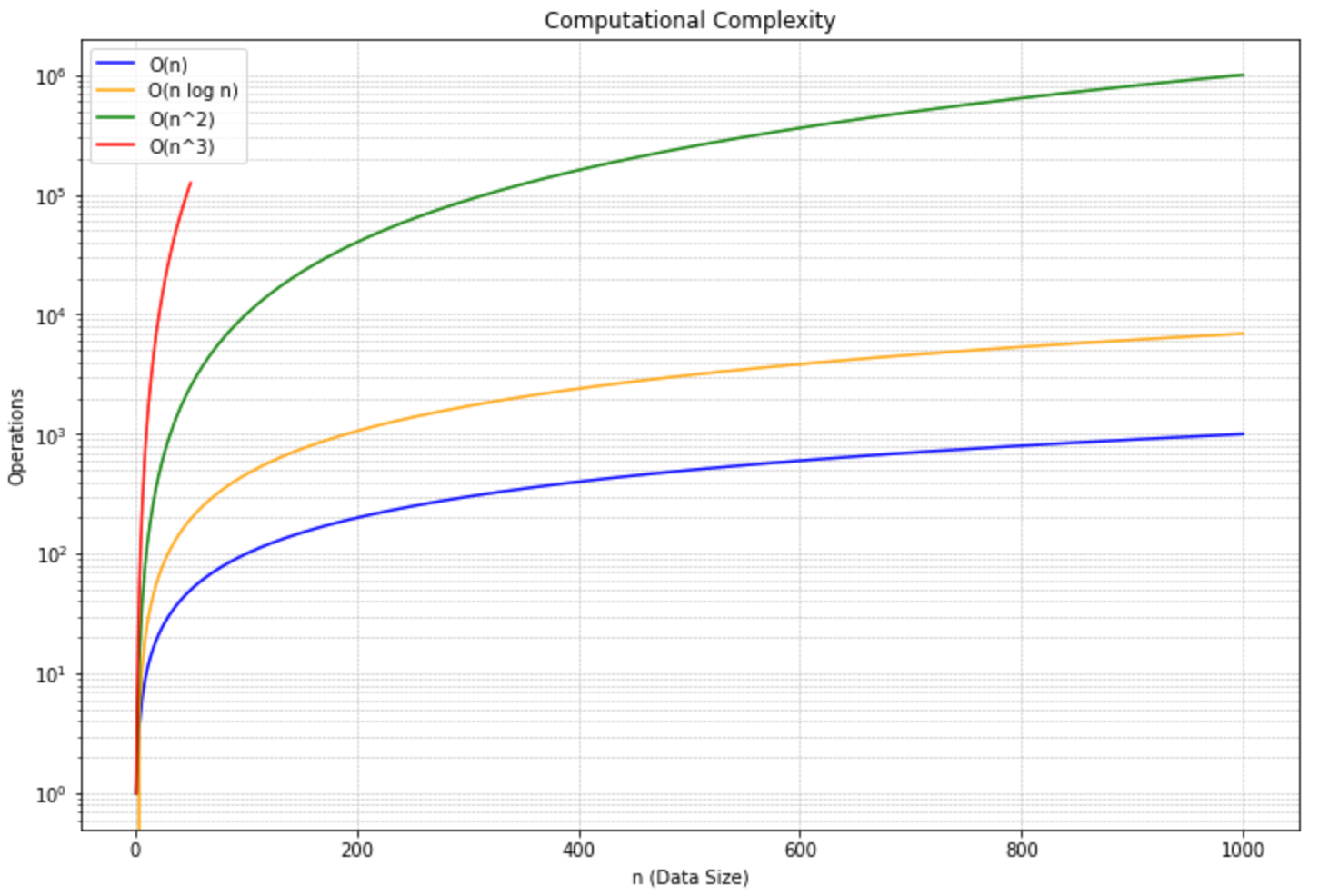
You can see that $O(n^3)$ is incredibly bad, but $O(n^2 \log n)$ is still not ideal.

For instance, consider an optimized approach that maintains a sorted list or a priority queue of distances:

# Hypothetical representation of optimized agglomerative approach
priority_queue = initialize_queue(data)
for i in range(n):
    closest_clusters = priority_queue.pop_smallest_distance()
    merge_clusters(closest_clusters)
    update_queue(priority_queue, data)

This optimization avoids the need to check every pair in every iteration. Instead, it efficiently identifies and merges the closest clusters. However, updating the priority queue and recalculating relevant distances can still take considerable time as the dataset grows.

Memory Usage

Hierarchical clustering, with its intricate methods, can be quite the space hog, demanding vast memory tracts that may not always be readily available.

At the heart of this memory challenge is the distance matrix. As we’ve seen, hierarchical clustering computes and stores distances between every pair of data points. This doesn’t just lead to complexity issues, it also leads to incredibly large arrays that need to be stored in memory.

import numpy as np
n = 1000000  # 1 million data points
# Initializing this matrix would be a memory behemoth
distance_matrix = np.zeros((n, n))

Consider a scenario with a million data points. The resulting matrix would be of the order of a trillion entries. A float64 NumPy array that size would require 7.45 terabytes of memory. Probably not doing that computation on your beat up macbook.

The memory demands don't stop at the distance matrix. As hierarchical clustering progresses, it produces a cascade of intermediate results. Especially in divisive clustering, where the data is recursively split into smaller clusters, storing these intermediate clusters and their associated data can add substantial memory overhead.

# Hypothetical representation of storing intermediate clusters in divisive clustering
all_clusters = []
current_clusters = initial_dataset_split(data)
while not is_base_case(current_clusters):
    all_clusters.append(current_clusters)
    current_clusters = further_split(current_clusters)

While hierarchical clustering's depth and detail are its strengths, they also contribute to its memory-hungry nature.

High-dimensional data exacerbates both computational and memory challenges. The "curse of dimensionality" makes distance measures less distinct in high-dimensional spaces, requiring more sophisticated methods or dimensionality reduction techniques. This in turn can impose additional computational overhead.

Techniques for Scaling Hierarchical Clustering

The scalability challenges of hierarchical clustering necessitate the development and adoption of techniques that can efficiently handle large or high-dimensional datasets. Various strategies have been introduced to address computational, memory, and quality concerns.

Sampling

One straightforward approach to manage large datasets is to work with a representative subset. By clustering a sample and then assigning the remaining data points to the closest clusters, the computational demands are substantially reduced.

from sklearn.utils import resample

# Assuming `data` is your dataset
sampled_data = resample(data, replace=False, n_samples=int(0.1 * len(data)))
# Hierarchical clustering can then be performed on `sampled_data`

While this approach reduces the dataset's size, it runs the risk of excluding potentially critical data points that could influence clustering outcomes.

Approximation Algorithms

Approximation algorithms play a pivotal role in offering a practical compromise in scenarios where obtaining the exact solution might be computationally prohibitive. Their primary goal is to deliver results that are close to the optimal, within an acceptable margin, while significantly reducing the computational effort.

The essence of approximation methods in hierarchical clustering lies in their ability to simplify the problem space. Instead of exhaustively considering all possible cluster combinations or distances, approximation methods utilize strategic shortcuts to derive a solution that's "good enough" in a fraction of the time.

One strategy involves constructing a Minimum Spanning Tree (MST) based on the distance matrix. The MST represents a subset of the edges from the complete graph that connects all data points without forming any cycles and has the minimum possible total edge weight.

By constructing and analyzing the MST, we can infer the hierarchy of clusters without directly working with the entire distance matrix. This method significantly reduces the time complexity, especially when paired with efficient algorithms for MST construction, such as Kruskal's or Prim's algorithms.

# Pseudocode representation of the MST-based approximation
def mst_based_clustering(data, distance_matrix):
    mst = construct_minimum_spanning_tree(distance_matrix)
    hierarchy = derive_hierarchy_from_mst(mst)
    return hierarchy

While MST-based and other approximation techniques expedite the clustering process, it's essential to understand the associated trade-offs. The reduced computational time often comes at the expense of solution accuracy. The derived clusters might not always match the quality or precision of those obtained through exhaustive methods.

Furthermore, the effectiveness of approximation methods can vary based on the nature and distribution of the data. It's crucial to evaluate the suitability of these algorithms in the context of the specific dataset and clustering objectives.

Divide and Conquer in Hierarchical Clustering

The divide and conquer strategy provides a structured approach to manage the computational and memory challenges associated with hierarchical clustering, especially for large datasets. By breaking the problem into smaller, more manageable sub-problems, this technique not only enhances efficiency but also offers modular control over the clustering process.

The dividing phase involves partitioning the dataset into smaller chunks or segments. Each of these chunks is of a manageable size, making the clustering process within each chunk computationally feasible and memory-efficient.

Once the data is partitioned, hierarchical clustering is applied individually to each chunk. As these chunks are smaller representations of the dataset, the clustering process within each segment is faster and demands less memory.

# Pseudocode for clustering individual chunks
def cluster_chunks(data, chunk_size):
    num_chunks = len(data) // chunk_size
    clusters = []
    for i in range(num_chunks):
        chunk = data[i * chunk_size: (i+1) * chunk_size]
        clusters_chunk = hierarchical_clustering(chunk)  # Placeholder function
        clusters.extend(clusters_chunk)
    return clusters

Post clustering, the clusters obtained from individual chunks might not represent the global structure of the entire dataset. Hence, there's a need to potentially merge clusters from different chunks. This merging phase is crucial to ensure that the localized clustering from individual chunks converges to a more holistic clustering representation of the entire dataset.

The divide and conquer strategy significantly reduces the time and memory requirements for hierarchical clustering. However, a crucial aspect to consider is the choice of chunk size and the merging criteria. In some ways with this approach, we’re back to the problem that hierarchical clustering solved—choosing parameters before we start instead of letting the algorithm work for us.

Reducing Dimensionality

For high-dimensional data, dimensionality reduction techniques like PCA (Principal Component Analysis) or t-SNE can be used prior to clustering. This can significantly reduce the computational burden.

from sklearn.decomposition import PCA

pca = PCA(n_components=50)  # Reduce data to 50 principal components
reduced_data = pca.fit_transform(data)

However, it's essential to ensure that the reduced representation retains the significant structures and relationships present in the original data.

Tools for Scaling Hierarchical Clustering

To work with the above techniques (or just brute force it), developers and researchers have produced tools and frameworks to help in scalable hierarchical clustering.

Software and Libraries

• Scipy: While Scipy's hierarchy module offers traditional hierarchical clustering methods, it has undergone optimizations over the years. The linkage algorithms, especially when combined with efficient data structures, can manage moderately large datasets with reasonable efficiency.

from scipy.cluster.hierarchy import linkage
Z = linkage(data, method='ward')

• Fastcluster: An optimized library for agglomerative clustering, fastcluster interfaces seamlessly with Scipy's hierarchical clustering but provides enhanced speed, especially beneficial for large datasets.

from fastcluster import linkage_vector
Z = linkage_vector(data, method='ward')

• HDBSCAN: This is an advanced clustering algorithm that builds upon DBSCAN and hierarchical clustering concepts. Particularly potent for data with varying cluster densities, HDBSCAN's implementation is optimized for performance.

  import hdbscan

clusterer = hdbscan.HDBSCAN()
labels = clusterer.fit_predict(data)

Distributed Systems

• Apache Spark MLlib: Spark's machine learning library, MLlib, includes scalable clustering algorithms that can be executed in distributed environments. By chunking datasets and processing them in parallel across nodes, Spark facilitates the clustering of extremely large datasets.

from pyspark.ml.clustering import BisectingKMeans
from pyspark.sql import SparkSession

spark = SparkSession.builder.appName("HierarchicalClustering").getOrCreate()
data_df = spark.read.format("libsvm").load("path_to_data")

bkm = BisectingKMeans().setK(2).setSeed(1)
model = bkm.fit(data_df)

• Dask: Similar to Spark, Dask enables parallel and distributed computing but retains an interface consistent with familiar tools like NumPy, pandas, and Scikit-learn. While Dask doesn't natively offer hierarchical clustering, its parallelism paradigms can be leveraged to implement custom scalable clustering solutions.

GPU Acceleration

The parallel processing capability of GPUs can be harnessed for clustering tasks. Libraries such as RAPIDS cuML provide GPU-accelerated machine learning algorithms, including clustering methods. These tools can drastically cut down computation times for large datasets.

import cuml.cluster
db = cuml.cluster.DBSCAN(eps=3, min_samples=2)
y_db = db.fit_predict(data)

Moving Beyond Naivety with Hierarchical Clustering

From computational and memory perspectives, naive implementations of hierarchical clustering quickly hit bottlenecks, driving the adoption of scalable techniques such as sampling, approximation, and distributed processing. Modern tools and frameworks, like Fastcluster, Apache Spark, and GPU-accelerated solutions, have emerged as invaluable assets, each catering to different parts of the scalability dilemma.

But the balance between efficiency and cluster quality is delicate, with potential repercussions in the outcomes of analyses. Choices, be it of distance metrics or linkage criteria, cast profound implications on the clustering results. In making these choices, analysts are back where they started, using heuristics in their data models that can shift the final analysis.

It is naive to think it could hierarchical clustering was a hands-free solution. Hierarchical clustering looks like it does all the work for you, until you give it a lot of work to do. Then its back on you as the analyst to know what you’re doing.