How to query a SQL database from Pandas

Most of the time, the data you want to work with in Pandas isn’t in a file on your desktop. All the good data usually lives in huge databases up in the cloud that you have to shout at in ALL UPPERCASE SQL COMMANDS like they’re hard of hearing.

So to get your data, you have to learn how to shout with Python, or in other words, how to use SQL commands in Python. We’ve already covered how to query a Pandas DataFrame with SQL, so in this article we’re going to show you how to use SQL to query data from a database directly into a Pandas DataFrame for easy manipulation, cleaning, and analysis.

For simplicity's sake, we’ll pick a publicly available dataset from Kaggle, about Airbnb Data in New York City.

Let's do this!

Step 1: Connecting to your dataset

Pandas has a built-in function to read from a database: read_sql. If you look through the docs for this function, you’ll see that it can take a ton of arguments:

pandas.read_sql(sql, con, index_col=None, coerce_float=True, params=None, parse_dates=None, columns=None, chunksize=None)

But really, you only need the first two: sql and con.

sql is, obviously, the SQL commands you are going to use to query your dataset. The shouty bit. The con is the connection. It is an open connection between the database and Python that Python can use to read and write data to or from the database. You have a few choices on how to set up your connection.

The most common option is to use SQLAlchemy. If you use Python code extensively to interact with your databases and want to concentrate on writing business logic and performant code, SQLAlchemy is the way to go. It provides a standard interface to handle database-agnostic code and boilerplate snippets to connect to various databases. It also offers object-relational mapping capabilities to use your data as business objects. If you have to do complex stuff to your dataset, like cascading updates or deletes between multiple tables, then use SQLAlchemy.

You set up a connection like this. First, install:

pip install sqlalchemy

Then import:

from sqlalchemy import create_engine

Then you use that create_engine function along with your database credentials (read more about those here) to build your connection:

engine_uri = f"mysql+pymysql://{username}:{password}@{hostname}/{database_name}"
connection = create_engine(engine_uri)

That connection (in this case to a MySQL database) would then be ready to use with read_sql.

That was pretty simple, but for this example we’re going to keep it even simpler. Instead of SQLAlchemy and an external database, we’re going to use a SQLite connection and a local SQLite database. SQLite is one of the most lightweight options to get started with SQL operations, since you don’t need to provision any servers. It’s standard, so you can perform most SQL querying operations and aggregations, and SQLite is also light (pun intended) on resources.

To read this data we need to first install sqlite3:

pip install sqlite3

Then import it:

import sqlite3

In this case, we've already got a .db file with our Airbnb data in it. We'll open a connection to that database using the connect function:

con = sqlite3.connect("Airbnb_Open_Data_schema")

With that connection as our con, we’re now ready to write our sql and use read_sql.

Step 2: Using read_sql to execute SQL queries in Python

Now that we have a connection established, we can treat Python like it's SQL. As we’re going to be using read_sql from Pandas, we need to install and import Pandas first:

pip install pandas
import pandas as pd

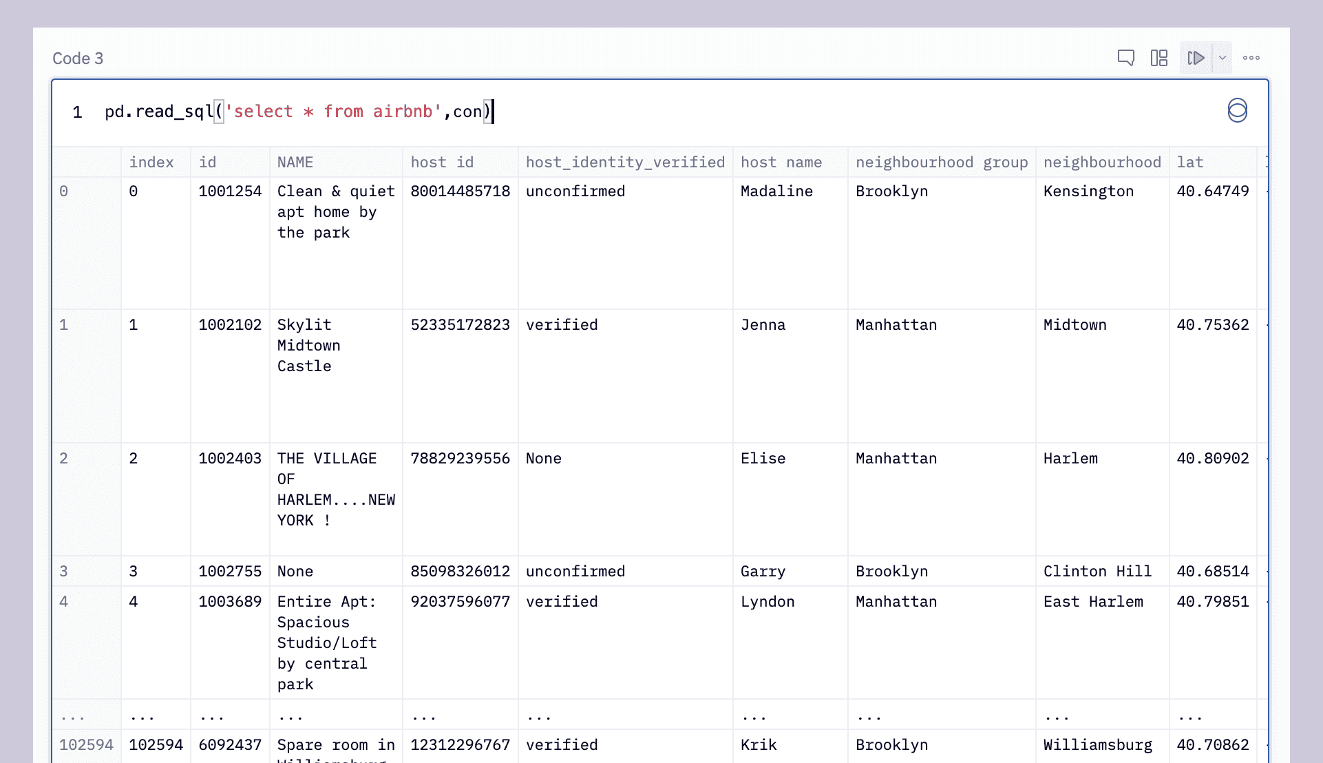
Let’s do an extremely basic query to get all our data:

pd.read_sql("select * from airbnb",con)

This outputs all 102,599 rows in the dataset:

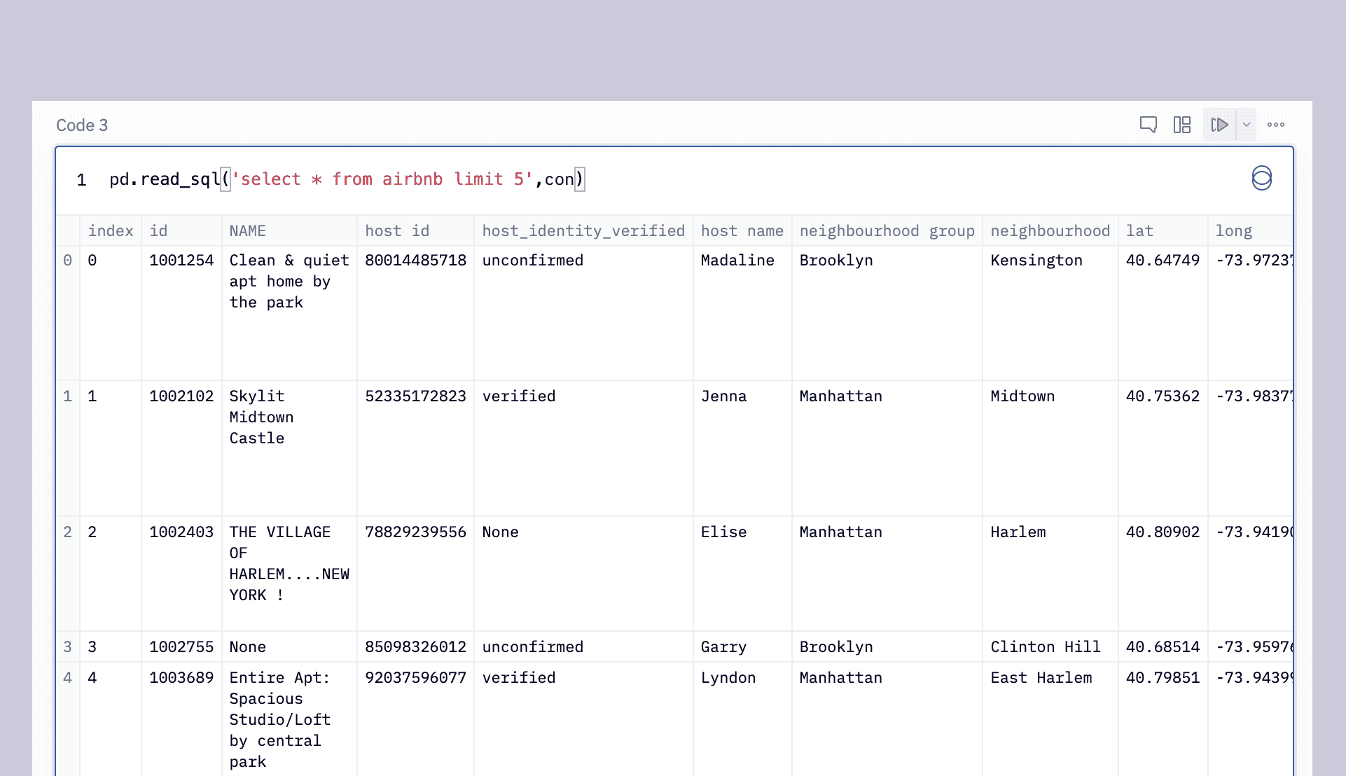
We can use the SQL limit clause to limit ourselves to just the first 5 rows, emulating df.head():

pd.read_sql("select * from Airbnb_Open_Data limit 5",con)

Which will output:

Since we’re using Pandas, the output is a DataFrame so we can get the same result with:

df = pd.read_sql("select * from Airbnb_Open_Data",con)
df.head()

This is the awesomeness of read_sql–you can combine the specificity of SQL with the power of Pandas.

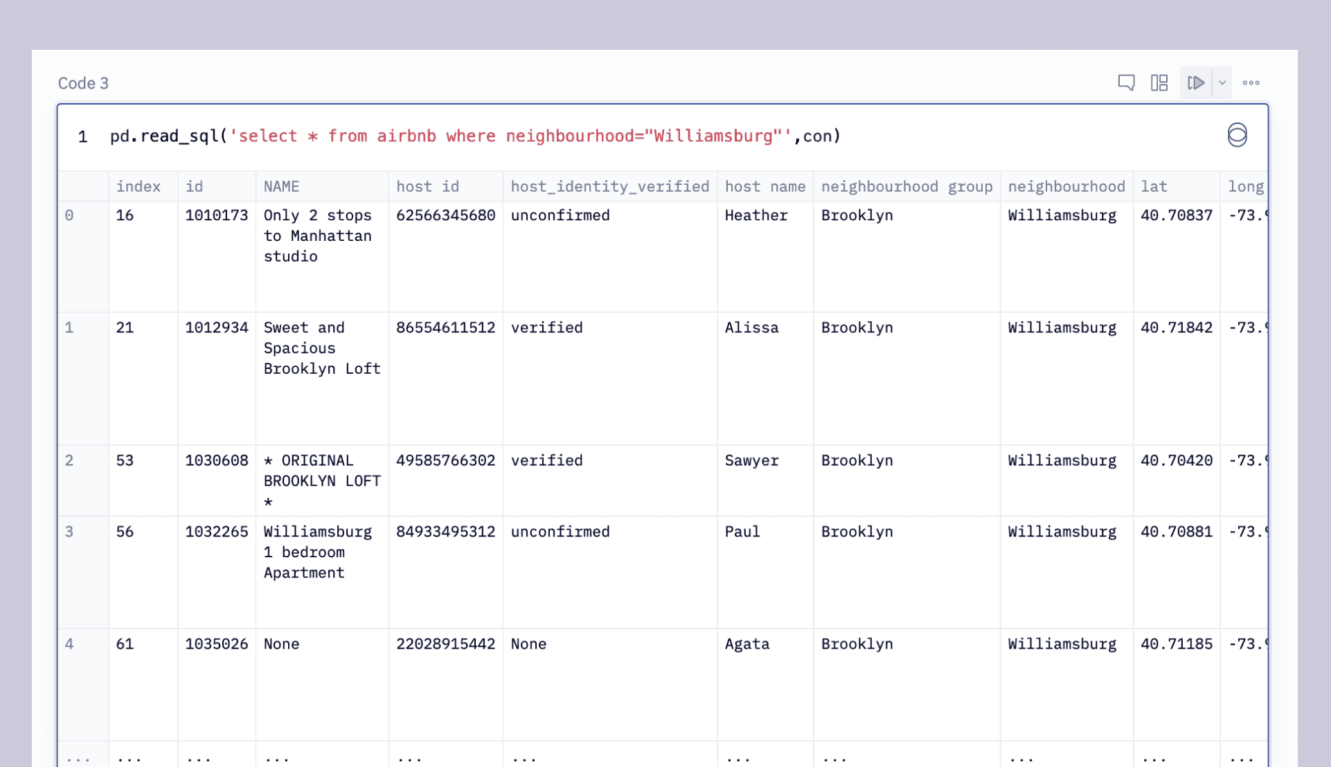
Going back to SQL for a moment, let’s build a couple of more helpful queries. We’re all hipsters (right?), so let’s get just the Airbnbs in Williamsburg:

pd.read_sql("select * from Airbnb_Open_Data where neighbourhood='Williamsburg'",con)

This outputs:

Or, using f-strings, we can iterate through a list of each of the five boroughs to get a count of Airbnbs in each:

boroughs = ['Manhattan', 'Brooklyn', 'Queens', 'Bronx', 'Staten Island']
for borough in boroughs:
   query = f"select * from Airbnb_Open_Data where neighbourhood_group='{borough}'"
   pd.read_sql(query,con)

Let’s say you want to get a list of all the Airbnbs in different price ranges. You can put the read_sql within a loop and use f-strings to build a new query with each iteration, such as:

for i in range(0, 1000, 100):
   query = f"select * from Airbnb_Open_Data where price between '${str(i)}' and '${str(i+99)}'"
   pd.read_sql(query,con)

Strings, numbers, dates–you can build all of these dynamically in Python and then query using SQL and read_sql.

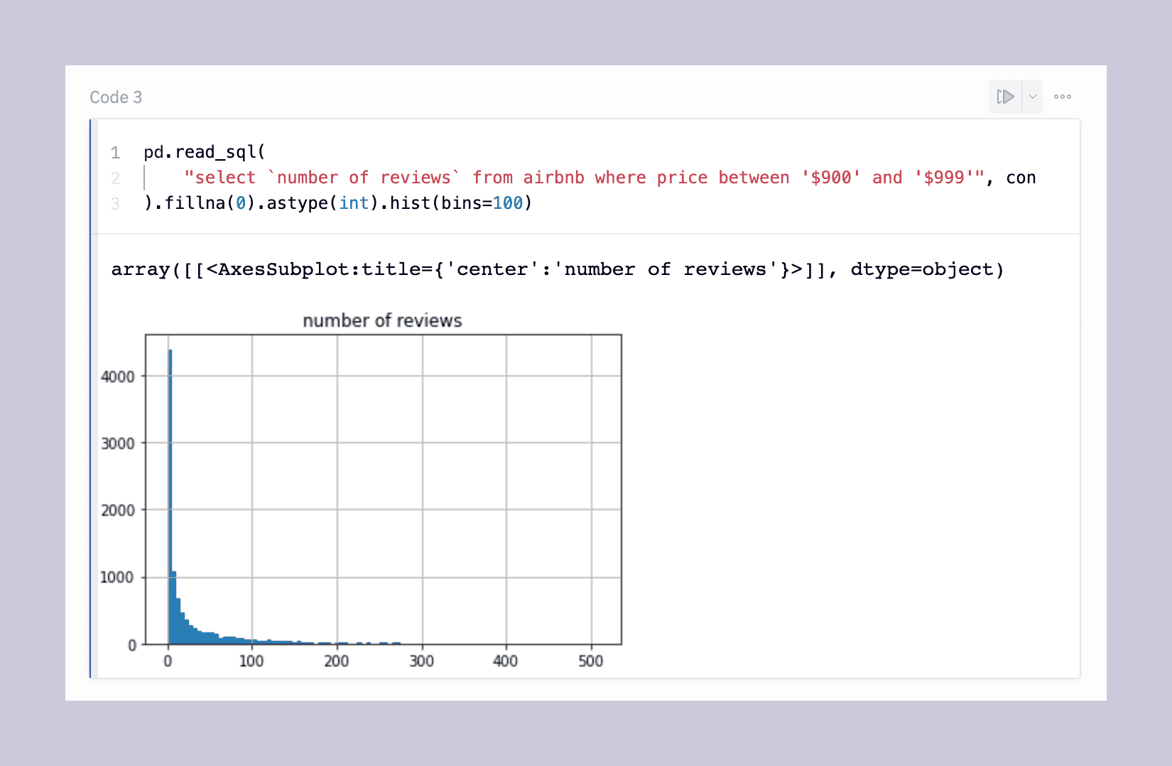
Finally, let’s use another nice facet of DataFrames: plotting. We can chain our SQL query with a plotting function for a one-line SQL-to-graph bonanza (with some data cleaning thrown in):

pd.read_sql("select `number_of_reviews` from Airbnb_Open_Data where price between '$900' and '$999'",con).fillna(0).astype(int).hist(bins=100)

This line:

• Get the number of reviews for all listings in the price range 900to999

• Cleans the data by filling any NaN fields with a 0

• Casts the reviews from a string to an int type

• Plots this data in a histogram with 100 bins

So you end up with this:

So with that one line, you can quickly see that most Airbnbs in this range have zero reviews, but the tail is long. Next steps in this analysis might be to cross-reference this data with the actual mean review rating for each property (maybe those are 270 one-star reviews…)

Wrapping up and next steps

Congratulations! You have gone through the initial building blocks of being able to query newly imported SQL data in Python. You now know the initial approach to query and filter your data and store them in DataFrames for further cleansing and processing, or even plot that data out straight from the database.

If you run into any issues with writing Panda functions for SQL querying, the community-driven Panda documentation and support should quickly help you get unstuck. If you want more options to write your queries in Python, we recommend checking our article about writing SQL in Python using Pandas.