Clustering, a fundamental task in machine learning, involves grouping data points based on their inherent similarities. Its goal is to ensure that data points in the same cluster are more similar than those in different clusters. They are employed extensively in numerous applications, clustering aids in data exploration, pattern recognition, and anomaly detection, among other tasks.
Three prominent data clustering algorithms frequently discussed in the literature are k-means, hierarchical clustering, and DBSCAN. While k-means and hierarchical clustering are rooted in partitioning and tree-based methodologies, DBSCAN operates on a density-based approach. The selection between these clustering algorithms often hinges on the characteristics of the dataset at hand and the desired outcomes from the clustering process.
Here, we want to look into the intricacies of these three clustering methods, comparing their methodologies, strengths, and limitations. If you want to follow along, all the code is in our Hex notebook here.
k-means Clustering
The k-means algorithm is one of the most widely recognized and implemented clustering techniques in machine learning. Its core principle revolves around partitioning a dataset into k distinct, non-overlapping clusters.
To understand the mechanics, consider a dataset X. The objective of k-means is to determine k centroids and assign each data point to the nearest centroid. These centroids, which represent the center of the clusters, are initialized randomly or based on specific heuristics.
The algorithm iteratively performs two primary steps:
- Assignment Step: Assign each data point in X to the nearest centroid. This assignment is typically based on the Euclidean distance, although other distance metrics can be employed.
- Update Step: Calculate the mean of the data points assigned to each centroid and set this mean as the new centroid.
This iterative process continues until the centroids no longer change significantly or a set number of iterations is reached.
Let's illustrate this using the iris dataset. First, we’ll load the dataset and visualize the data:
import pandas as pd
import matplotlib.pyplot as plt
import seaborn as sns
from sklearn import datasets
# Load the iris dataset
iris = datasets.load_iris()
data = iris.data
target = iris.target
feature_names = iris.feature_names
target_names = iris.target_names
# Visualize the data
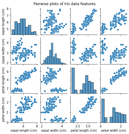
sns.pairplot(pd.DataFrame(data, columns=feature_names), height=1.5)
plt.suptitle('Pairwise plots of Iris data features', y=1.02)
plt.show()The pairwise plots give us a visual representation of the relationships between the different features of the Iris dataset. Some feature combinations seem to form distinct clusters.
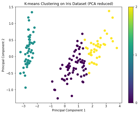
For K-means clustering, we'll need to specify the number of clusters k. Given that the Iris dataset has three species, we'll set k=3. After clustering, we'll visualize the results on the first two principal components for simplicity.
from sklearn.cluster import KMeans
from sklearn.decomposition import PCA

# Apply KMeans clustering
kmeans = KMeans(n_clusters=3, random_state=42)
kmeans_clusters = kmeans.fit_predict(data)

# Reduce data to 2D using PCA for visualization
pca = PCA(n_components=2)
reduced_data = pca.fit_transform(data)

# Plot the clustered data
plt.figure(figsize=(8, 6))
scatter = plt.scatter(reduced_data[:, 0], reduced_data[:, 1], c=kmeans_clusters, cmap='viridis', s=50)
plt.title('K-means Clustering on Iris Dataset (PCA reduced)')
plt.xlabel('Principal Component 1')
plt.ylabel('Principal Component 2')
plt.colorbar(scatter, ticks=[0, 1, 2])
plt.show()
The visualization shows the results of K-means clustering on the Iris dataset reduced to two principal components. The three clusters are visibly distinct, which is a good sign.
While k-means is computationally efficient and works well for datasets where the clusters are approximately spherical, it has its limitations. One of the inherent challenges is the need to specify the number of clusters, k, in advance. The algorithm is also sensitive to the initial placement of the centroids, leading to possible convergence to a local optimum. To mitigate this, multiple runs with different centroid initializations are recommended. Furthermore, k-means assumes clusters to be of roughly equal sizes and can be biased towards globular shapes, which may not always represent the underlying distribution of data points.
Suitable Scenarios for k-means:
If you're dealing with a large dataset and need a method that balances accuracy with computational efficiency, k-means is often a strong contender. Its linear time complexity in terms of the number of data points makes it a scalable solution.
Also, k-means is particularly effective when there's a preliminary understanding or estimation of how many clusters the dataset should be segmented into. As mentioned earlier, techniques like the Elbow method can assist in such determinations.
Moreover, datasets that inherently have a globular cluster shape are ideal candidates for k-means. The algorithm naturally segments data into spherical clusters, making it well-suited for such distributions.
Hierarchical Clustering
Hierarchical clustering is a method that seeks to build a hierarchy of clusters either through a bottom-up or top-down approach. In contrast to k-means, which partitions data into distinct clusters, hierarchical clustering creates a tree of clusters, offering multiple levels of granularity.
The bottom-up approach, known as agglomerative clustering, starts by treating each data point as a single cluster and then successively merging the closest pairs of clusters. This process repeats until only one large cluster remains, encompassing all data points.
On the other hand, the top-down approach, called divisive clustering, begins with all data points in a single cluster and then proceeds to divide them into smaller clusters until each data point forms its own cluster.
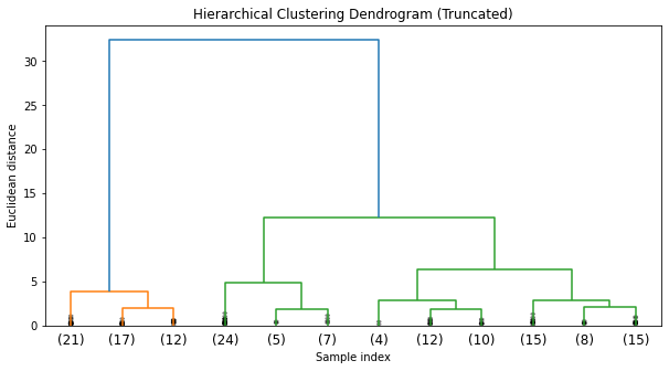
One of the notable outcomes of hierarchical clustering is the dendrogram, a tree-like diagram that illustrates the sequence of merges or splits. This visualization can be particularly useful in understanding the hierarchical structure of data.
We'll use the agglomerative clustering method. We'll visualize the resulting dendrogram to decide on an appropriate cut-off for the number of clusters.
from scipy.cluster.hierarchy import dendrogram, linkage
from sklearn.cluster import AgglomerativeClustering
# Compute the linkage matrix for hierarchical clustering
Z = linkage(data, 'ward')
# Plot the dendrogram
plt.figure(figsize=(10, 5))
dendrogram(Z, truncate_mode='lastp', p=12, show_leaf_counts=True, show_contracted=True)
plt.title('Hierarchical Clustering Dendrogram (Truncated)')
plt.xlabel('Sample index')
plt.ylabel('Euclidean distance')
plt.show()
# Apply Agglomerative Clustering based on the dendrogram
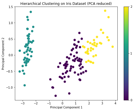
agglo_clusters = AgglomerativeClustering(n_clusters=3).fit_predict(data)
# Plot the clustered data
plt.figure(figsize=(8, 6))
scatter = plt.scatter(reduced_data[:, 0], reduced_data[:, 1], c=agglo_clusters, cmap='viridis', s=50)
plt.title('Hierarchical Clustering on Iris Dataset (PCA reduced)')
plt.xlabel('Principal Component 1')
plt.ylabel('Principal Component 2')
plt.colorbar(scatter, ticks=[0, 1, 2])
plt.show()The dendrogram from the hierarchical clustering suggests that a cut at three clusters would be appropriate, given the large distances between the merges at that level. This aligns with our prior knowledge that there are three species in the Iris dataset.
The PCA visualization also shows three distinct groups, similar to the K-means clustering result.
Distance metrics (e.g., Euclidean, Manhattan) and linkage criteria (e.g., single, complete, average, ward) play a pivotal role in the clustering process. The chosen distance metric calculates the dissimilarity between data points, while the linkage criterion determines the distance between clusters, guiding the merge or split decisions.
While hierarchical clustering is adept at revealing data structures and is not constrained by a pre-specified number of clusters, it does have drawbacks. The method's computational complexity tends to make it less suited for large datasets. Moreover, decisions made in early stages, such as merging two clusters, cannot be undone, potentially leading to suboptimal results if the initial choices were not accurate reflections of the data's intrinsic structure.
Suitable Scenarios for Hierarchical Clustering:
Hierarchical clustering shines in exploratory data analysis. When diving into a dataset, understanding its inherent hierarchical structure can offer significant insights that other clustering techniques might overlook.
Given its computational characteristics, hierarchical clustering is best suited for smaller datasets. The algorithm typically has a higher computational overhead compared to methods like k-means, making it less ideal for extensive datasets but more apt for ones where the computational load is manageable.
If your analysis demands multiple levels of clustering granularity, hierarchical clustering is a wise choice. The nested partitions it produces offer a range of segmentation levels, catering to diverse analytical needs.
Hierarchical clustering remains a powerful tool in the machine learning arsenal, particularly for exploratory data analysis where the multi-level clustering representation can shed light on underlying patterns.
DBSCAN
DBSCAN is a density-based clustering algorithm that segregates data points into high-density regions separated by regions of low density. Unlike k-means or hierarchical clustering, which require specifying the number of clusters beforehand, DBSCAN automatically determines clusters based on the density of data points.
The fundamental concepts driving DBSCAN are core points, border points, and noise points:
- Core Points: A point is considered a core point if there are at least MinPts number of points (including itself) within a radius ε of it.
- Border Points: These are points that are not core points themselves but fall within the ε radius of a core point.
- Noise Points: Points that are neither core nor border points. These are often outliers or data points in low-density regions.
The DBSCAN algorithm works as follows:
- Start with an arbitrary point. If there are MinPts within ε distance of this point, establish a new cluster and include all points within this distance.
- Expand the cluster by checking all points within ε distance of every point in the cluster. If any of these new points have at least MinPts within ε distance of them, add them to the cluster.
- Continue the process until no more points can be added to the cluster. Then, move on to the next unvisited point and repeat the process.
- Points that don't belong to any cluster are labeled as noise.
Let's apply DBSCAN to the Iris dataset and visualize the results.
from sklearn.cluster import DBSCAN

# Apply DBSCAN clustering
dbscan = DBSCAN(eps=0.5, min_samples=5)
dbscan_clusters = dbscan.fit_predict(data)

# Plot the clustered data
plt.figure(figsize=(8, 6))
scatter = plt.scatter(reduced_data[:, 0], reduced_data[:, 1], c=dbscan_clusters, cmap='viridis', s=50)
plt.title('DBSCAN Clustering on Iris Dataset (PCA reduced)')
plt.xlabel('Principal Component 1')
plt.ylabel('Principal Component 2')
plt.colorbar(scatter)
plt.show()

# Return the unique cluster labels
unique_labels = np.unique(dbscan_clusters)
unique_labels
The DBSCAN clustering has identified clusters in the Iris dataset, and the visualization shows the distribution of these clusters on the first two principal components.
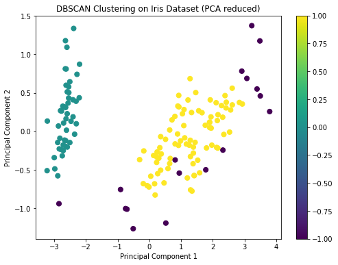
DBSCAN identified two main clusters and some noise points. This is a bit different from the K-means and hierarchical clustering results, which identified three clusters. This discrepancy can arise because DBSCAN is more sensitive to density variations and might treat sparse regions as noise.
DBSCAN's strengths lie in its ability to identify and handle noise, discover clusters of varying shapes, and its independence from having to predefine the number of clusters. However, it can face challenges when clusters have different densities, as a single set of ε and MinPts values might not suit all clusters. Additionally, the algorithm's performance can vary based on the chosen distance metric.
Suitable Scenarios for DBSCAN
DBSCAN excels in environments where the dataset contains significant noise or irrelevant data points. Since it inherently categorizes less dense regions as noise, it can produce cleaner clusters in such scenarios.
If your data exhibits non-globular or irregularly shaped clusters, DBSCAN is often a more fitting choice than centroid-based methods. It doesn't rely on the mean or median of points and instead focuses on the density, allowing it to contour around data naturally.
Spatial datasets, where the proximity and density of data points carry significance, align well with DBSCAN's capabilities. Its foundation on spatial density makes it an appropriate choice for geospatial clustering or when working with spatially-coherent data.
Comparing the Methods
Input Parameters
One of the first aspects to consider when choosing a clustering algorithm is the type and nature of the input parameters.
In k-means, the primary parameter is k, which signifies the number of clusters to be formed. Its choice can significantly influence the clustering outcome. One common technique to determine a suitable k is the Elbow method, which involves plotting the variance as a function of the number of clusters, and selecting the 'elbow point' where adding more clusters does not significantly decrease the variance.
DBSCAN, on the other hand, requires two primary parameters: ε, the radius that determines the neighborhood around a data point, and MinPts, the minimum number of points needed to form a dense region. The selection of these parameters is critical and can influence the quality of the clusters.
Hierarchical clustering's primary concern is the choice of distance metric (like Euclidean, Manhattan) and linkage criteria (single, complete, average, ward). The distance metric defines how the similarity between two data points is calculated, while the linkage criterion determines how pairs of clusters are merged or split.
Shape of Clusters
Different clustering algorithms show varied biases towards the shape of the clusters they form.
k-means tends to bias towards spherical clusters due to its reliance on the centroid and distance-based calculations. This might not capture more complex cluster shapes effectively.
DBSCAN, on the contrary, can find arbitrarily shaped clusters. Its density-based nature allows it to adapt to the structure of the data, forming clusters that might be intertwined or elongated.
For hierarchical clustering, the shape and structure of clusters largely depend on the linkage criteria. For example, single linkage might lead to elongated, 'chain-like' clusters, while complete linkage tends to create more compact, rounder clusters.
Handling of Noise and Outliers
Noise and outliers can considerably distort clustering results.
k-means is sensitive to noise and outliers since it uses centroids. A few outlying points can significantly shift the position of centroids, leading to suboptimal clusters.
DBSCAN inherently identifies and separates noise from clusters. Points that don't belong to any cluster are labeled as noise, which can be highly beneficial when working with messy real-world data.
Hierarchical clustering, particularly with single linkage, is susceptible to noise and outliers. This is because a single outlying point can lead to the creation of a long chain, affecting the overall clustering structure.
Scalability
Regarding scalability, k-means often emerges as a winner due to its linear time complexity in the number of data points. Especially with the Elkan's or Hamerly's accelerated variants, k-means can handle large datasets with efficiency.
DBSCAN, while linear in nature, can become computationally expensive if the neighborhood search isn't optimized. Techniques such as KD-Tree or Ball-Tree can be employed to speed up the neighborhood search, making DBSCAN more scalable.
Hierarchical clustering, particularly the agglomerative approach, typically has a time complexity of O(n^3) but can be reduced to O(n^2 \log n) with efficient data structures. Still, it remains less scalable than k-means or DBSCAN for very large datasets.
Determining the Number of Clusters
The need to pre-specify the number of clusters is a key consideration.
With k-means, k has to be defined in advance. As mentioned earlier, methods like the Elbow technique can assist in determining an optimal k.
DBSCAN inherently determines the number of clusters based on data density. There's no need to specify the number of clusters beforehand, which can be advantageous when the clustering structure is unknown.
In hierarchical clustering, the dendrogram provides insights into potential cluster formations. Cutting the dendrogram at various heights allows us to choose different numbers of clusters, providing flexibility in determining the cluster count.
Choosing your approach
In data clustering, there is no one-size-fits-all solution. The dataset at hand, combined with the specific goals of the clustering task, play pivotal roles in determining the most fitting clustering technique.
Selecting the right clustering method requires a blend of domain knowledge, understanding of the data's characteristics, and awareness of each method's nuances. As clustering continues to evolve with advancements in machine learning and data science, it remains a potent tool in any data scientist's toolkit. By appreciating the strengths and limitations of each method, we position ourselves to make informed and impactful clustering decisions in our analytical endeavors.
If this is is interesting, click below to get started, or to check out opportunities to join our team.