Blog

Accessing Data in Jupyter with Python

Learn how to access the most popular data sources with Python in Jupyter Notebooks

Andrew Tate

Getting started with Accessing Data in Jupyter

The most popular data sources that are widely used across the industries to access the data are:

Files: CSV, Excel, JSON, TXTs, and Pickle, that can store structured and unstructured data. These files are stored in local or cloud storage and can be accessed using Python in Jupyter.
Databases and Data warehouse: Data can be stored in different relational and non-relational databases and data warehouses such as MySQL, PostgreSQL, MongoDB, Redshift, and Snowflake.
APIs: Data can also be accessed through APIs from multiple endpoints that sometimes may or may not need authentication.
Dataset Repositories: Finally, different platforms provide open source datasets for ML and AI tasks such as Kaggle, Data.world, or Hugging Face. You can load data directly from these platforms.

For this tutorial, we will use the Python 3.10 language and a Jupyter Notebook for writing the code. You can install Python from the official website or you can download the Anaconda distribution that comes with preinstalled Python and a set of useful Python libraries. Also for downloading Python packages (libraries), you can use either Python Package Manager (PIP) or Conda. Finally, the code that we are going to develop in this tutorial will be platform-independent.

Installing and Creating a Jupyter Notebook

To begin with, you can install one of the Jupyter flavors: Jupyter Notebook or Jupyter Lab. If you are using the Anaconda distribution then you can skip this part as it already comes with Jupyter Notebook and Jupyter Lab preinstalled.

But, if you have installed Python standalone from the official website then you need to install the Jupyter Notebook or Lab with the help of either PIP as follows:

# to install jupyter notebook
pip install notebook

# to install jupyter lab
pip install jupyterlab

Once the Jupyter notebook is installed, you can run Jupyter notebook in the terminal to start your notebook instance. This notebook instance will open in your default browser when you run the above command, if does not open automatically then copy the URL and paste it into your favorite browser to open the notebook server.

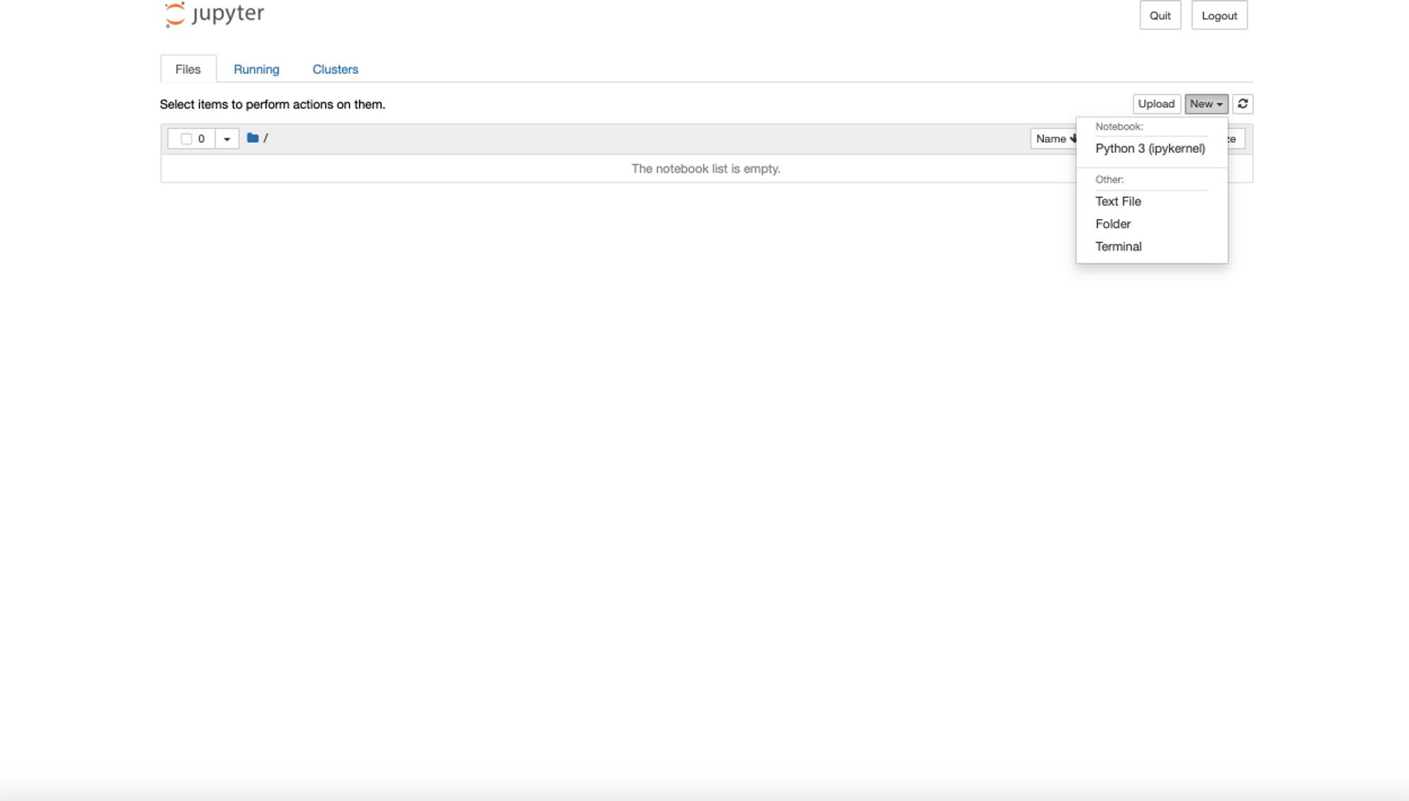
Next, to open a notebook for the experiment, click on the New > Python (Ipykernel) option.

Now a fresh notebook will be open for you to experiment and load data from multiple sources.

Installing Necessary Dependencies

Python provides a list of dependencies to develop different solutions with ease. For loading the data in Python, one most important libraries is Pandas which helps you load data from multiple data sources. You can install pandas using PIP as follows:

$ pip install pandas

For loading the data from the APIs or websites you will also require the requests package which can be downloaded as follows:

$ pip install requests

Note: We will need some other libraries that we will install as part of upcoming sections.

This is it, you are now all ready to load the data from multiple data sources. For this article, we will be using the most popular Iris dataset that can be downloaded online with multiple file extensions.

Accessing Data from Files

Using these data file formats such as CSV, JSON, Excel, or text files brings simplicity in saving and loading data and improves the portability of data. The downsides to these formats is that they may not be optimal for handling large-scale datasets, lack built-in support for complex data structures or relationships, and can sometimes suffer from inefficiencies in terms of read/write speeds compared to binary or database storage formats.

The pandas library from Python allows you to access the data from all major file types along with different exploration and visualization options.

Let’s start with importing pandas that we’ll use throughout this article.

# import dependency
import pandas as pd

Reading Data from Excel Files

Excel files are used to store tabular data and can have more than one sheet to store different relational tables. Excel (or Google Sheets) is incredibly powerful and common in business, so analysts might find a file given to them for analysis. Pandas provides the read_excel() method to load the data from Excel files. You can load different sheets of data from Excel into the Jupyter environment.

Note: Every time you load the data from any file type, it is always loaded as a DataFrame, a data structure of Pandas for storing the tabular or relational data.

An example of loading the iris data Excel file may look like this:

# excel absolute file path
excel_file = 'Datasets/iris.xls'

# read data from an excel file
iris_xl_data = pd.read_excel(excel_file, sheet_name='Data')

# check the first few rows of data loaded from Excel
iris_xl_data.head()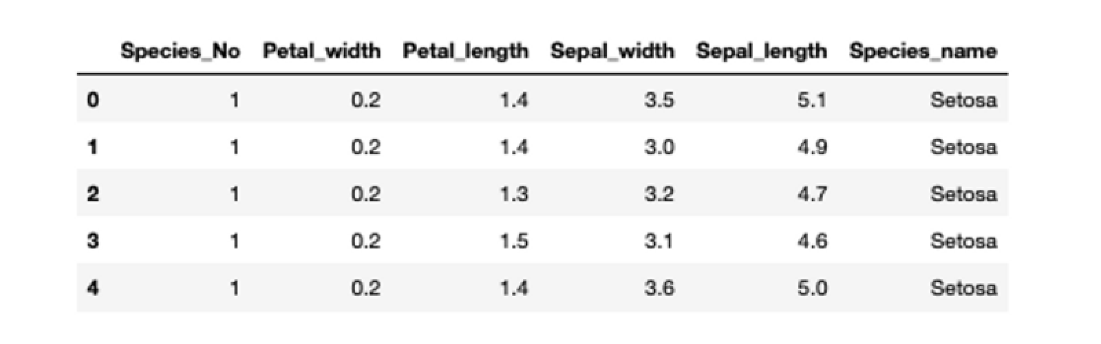

Note: You can specify the absolute or relative path of files in any pandas read data function.

As you can observe, we have specified the sheet_name that tells the Pandas to load the data from a specific Excel sheet. Other arguments of the read_excel() method you might want to use are:

header: Row (0-indexed) to use for the column labels. By default, it is inferred, but you can set it to None if there's no header.
names: This is a list corresponding to the column names. Use this if you want to override or set column names.
usecols: A list of columns or column range (e.g., 'A:D') to import from the Excel file.
dtype: Dict of column name to data type. If not provided, pandas will try to infer the data type.

Reading Data from CSV Files

CSV files are mainly used for storing relational data and are quick and easy to use with Python and Jupyter. Pandas provides the read_csv() function that can load the data in any environment and provides features to analyze and visualize the loaded data. A sample code to load the iris CSV file using Pandas will look like this:

# csv file path
csv_file = 'Datasets/iris.csv'

# load data from the CSV file
iris_csv_data = pd.read_csv(csv_file)

# check the first few rows of data loaded from CSV
iris_csv_data.head()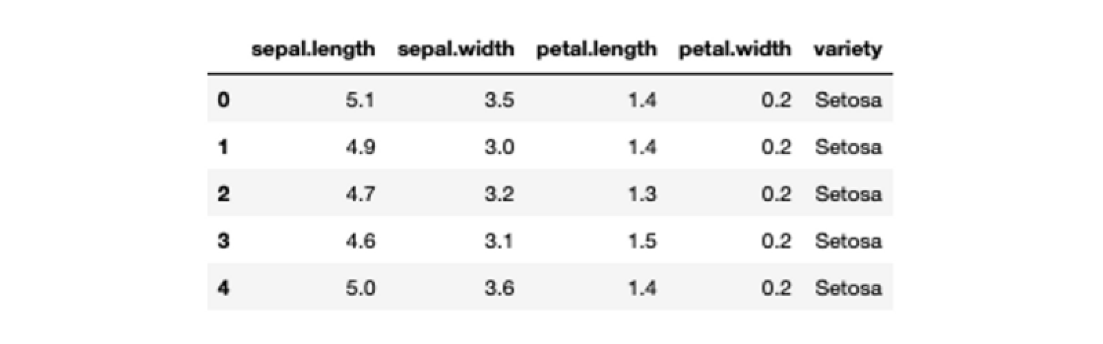

The read_csv() function also supports different arguments to:

Load specific columns:

df = pd.read_csv('filename.csv', usecols=['column1', 'column2'])

Skip erroneous rows:

df = pd.read_csv('filename.csv', error_bad_lines=False)

Break files into chunks:

chunk_iter = pd.read_csv('filename.csv', chunksize=10000)

To learn more, you can check the official page.

Reading Data from JSON Files

JSON is a simple, lightweight, and widely used data format that stores data in human-readable format. It uses key-value pairs where each key is a string that uniquely identifies a value, which can be a string, number, boolean, array, or another JSON object. This format is commonly used for configuration files, responses from APIs, and data storage in various applications and is well suited for storing small-size dataset features.

Pandas provide the read_json() method that helps you load the JSON files into a Dataframe. An example to load the iris.json file using pandas will look like this:

# JSON file path
json_file = 'Datasets/iris.json'

# load data from the JSON file
iris_json_data = pd.read_json(json_file)

# check the first 5 rows of data loaded from JSON
iris_json_data.head()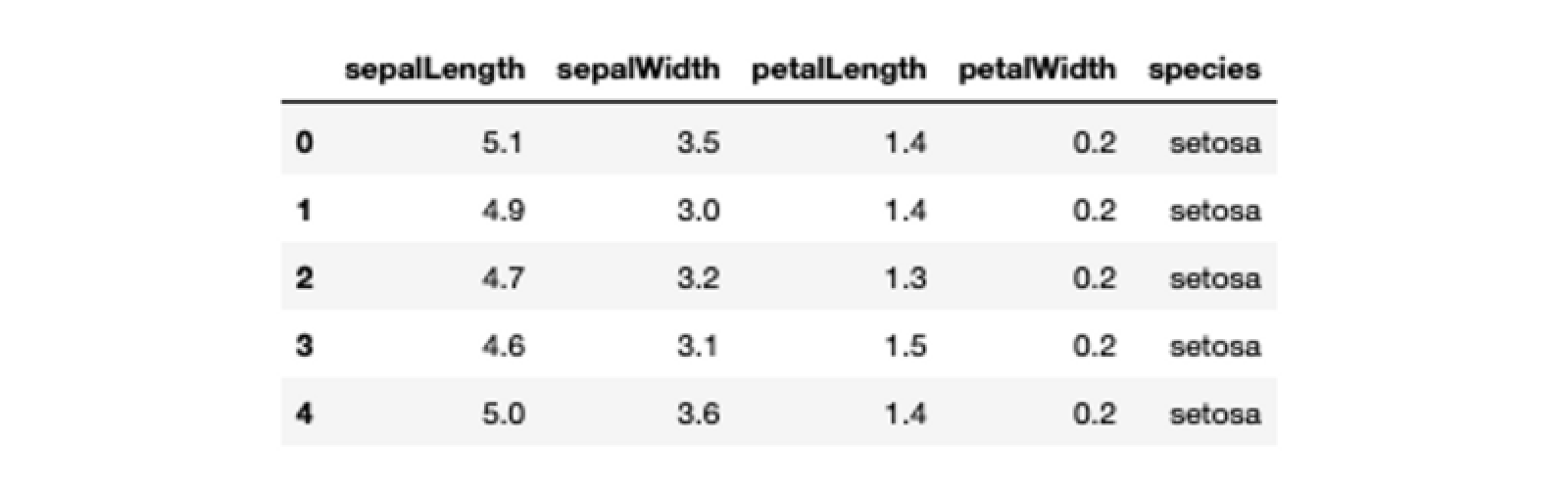

A helpful parameter for read_json() is the orient parameter. The orient parameter specifies the expected format of the JSON string or file. Using the correct orient value is crucial to ensure that the JSON data is read correctly into a DataFrame. For instance, if your JSON file was formatted:

[
{"X": 1, "Y": 2},
{"X": 3, "Y": 4},
{"X": 5, "Y": 6}
]

Then you would want to set orient to records. Whereas if your data was formatted:

{
"A": {"X": 1, "Y": 2},
"B": {"X": 3, "Y": 4},
"C": {"X": 5, "Y": 6}
}

You would set it to index. read_json() will try to infer the structure, but this parameter makes it explicit. You can learn more about loading JSON files with different arguments from the docs.

Pandas also supports file formats such as XML, HDF5, HTML, LaTeX, Fixed-Width txt files, and others. You can check all of them here.

Accessing Data From Databases and Data Warehouses

While file storage is good for small-size datasets, databases, and data warehouses are designed to hold almost any size of data. Most organizations store their large amount of business-specific data in local or cloud databases such as MySQL, MongoDB, or PostgreSQL.

These databases are normally created, accessed, and managed using the Structured Query Language (SQL) for different business purposes. Python provides a lot of connectors to access the data from different types of databases using the same SQL queries. Again, pandas play a key role as you can read the queried data as a dataframe and perform multiple operations of your choice.

Accessing Data from SQLite DB

SQLite is a C language library that is used to implement lightweight disk-based databases that are small, fast, self-contained, and highly reliable. This makes it popular across organizations for regular application development as these databases don’t require a separate server process and can be directly integrated into applications.

Python provides the sqlite3 module that can help you interact with SQLite databases. You don’t need to install this dependency as it already comes preinstalled with Python>2.5. To select data from the SQLite database the code will look like this:

# import dependency
import sqlite3 as sql

# create a connection to the database and a cursor to execute queries
conn = sql.connect('/Path_to/database_file.db')
cur = conn.cursor()

# query data from database
query = "SELECT * FROM tablename"
results = cur.execute(query).fetchall()

# create a DataFrame from the DB data
df = pd.DataFrame(results)

# Close the cursor and connection
cur.close()
conn.close()

In the above code, we have first created a connection with the SQLite database by providing the path of the DB file to the connect() method. Then we executed an SQL query to select the data from DB using the execute() method. Finally, the queried data is passed to the pandas DataFrame() method to be read as a DataFrame object. Do not forget to close the connection once your work is done.

Accessing data from a SQL database mostly involves manipulating the SQL query itself. Here, we’re getting all the data from the table, but a few other ways to query select data might be:

Filtering Data Using WHERE:

SELECT column1, column2
FROM tablename
WHERE column1 = 'some_value';

Sorting Data with ORDER BY:

SELECT column1, column2
FROM tablename
ORDER BY column1 DESC;   -- DESC for descending, ASC for ascending (which is default)

Limiting Results with LIMIT:

SELECT column1, column2
FROM tablename
LIMIT 10 OFFSET 20;  -- Skips the first 20 records and fetches the next 10.

Fetching Unique Records with DISTINCT:

SELECT DISTINCT column1
FROM tablename;

Depending on the specific SQL database flavor (e.g., MySQL, PostgreSQL, SQLite, SQL Server), there may be additional functions and syntax variations available.

Accessing Data from PostgreSQL DB or Data warehouses

Python provides options to connect with different relational and non-relational databases, and data warehouses to help manage them. You can access the data from these databases using the psycopg2 module which helps you to connect with a variety of databases and data warehouses. You can use PIP to install psycopg2 package as follows:

$ pip install psycopg2

To access data from a PostgreSQL database following code can be used:

# import dependency
import psycopg2

# create a connection to the database
conn = psycopg2.connect(
	host = "localhost",
	user = "yourusername",
	password = "yourpassword",
	database = "yourdatabase"
)

# select data from DB table
query = "SELECT * FROM tablename"
df = pd.read_sql_query(query, conn)

# close connection
conn.close()

First, you need to provide the necessary details such as the host and port where the DB is running, the username and password of the DB, and finally the name of the DB to establish a connection.

Then you can write the desired SQL query to operate on the data for example accessing the data. Pandas read_sql_query() helps you read data from different databases and warehouses and requires only the query and connection parameters. Once the dataset is loaded as a dataframe, close the connection to the database.

Accessing Data from MySQL DB

MySQL is one of the widely used relational database management systems that is used to store tabular data. Many organizations use this DB to store business data for different purposes due to its performance, reliability, and versatility. Python provides a lot of connector modules to connect to MySQL, one of them is mysql-connector. It can be downloaded using PIP as follows:

$ pip install mysql-connector

Similar to other DBs, you need to first establish a connection with the DB, access the data, and close the connection once your task is done.

# import mysql dependency
import mysql.connector

# create a connection to the database
conn = mysql.connector.connect(
	host="localhost",
	user="yourusername",
	password="yourpassword",
	database="yourdatabase"
)

# select data from DB table
query = "SELECT * FROM tablename"
df = pd.read_sql(query, conn)

# close connection
conn.close()

Accessing Data with APIs

If data is coming from a source outside your organization, you’ll need to access the data using APIs. The process starts with sending a request containing different query parameters and access credentials to the endpoint (the platform that contains the data).

When the credentials and query parameters are validated, the endpoint returns a response such as response code and the data you wanted to access (usually in JSON format) otherwise it will throw an error.

When working on Python, the requests module helps you access the data using APIs of different platforms in the Jupyter environment.

Accessing Data with APIs without Credentials

Sometimes data can be accessed without any credentials using public APIs. A simple example of reading the JSON data from a URL using the get() method from the requests library will look like this:

# Import necessary libraries
import requests

# Specify the URL where the dataset is hosted
url = "<https://raw.githubusercontent.com/gouravsinghbais/Accessing-Data-in-Jupyter/master/Dataset/iris.json>"

# Send an HTTP GET request to the specified URL
response = requests.get(url)

# Print the HTTP status code (e.g., 200 for "OK", 404 for "Not Found")
print(response.status_code)

# Print the JSON content of the response
print(response.json())

# Convert the JSON response to a pandas DataFrame
res = pd.DataFrame(response.json())

# Display the first 5 rows of the DataFrame
res.head()

Here, you only need a URL to access the JSON data. The response has two parts to it, one is the response code and the other is the JSON body that contains the data. The JSON data can be read directly as a dataframe using the Pandas module.

Accessing Data with APIs with Credentials

Often data will be protected and require specific credentials to authenticate your identity. You may also want to request the specific data for which some additional query parameters can be required. The same get() method can be used here as well where you can also pass the additional parameters as follows:

# Import the necessary libraries
import requests

# Define the parameters for the API request
parameters = {
    "personal_api_key": "YOUR_API_KEY",  # Replace with your actual API key
    "date": "2021-09-22"                 # The date for which you want data
}

# Send an HTTP GET request to the specified URL with the given parameters
response = requests.get(url, params=parameters)

# Print the HTTP status code (e.g., 200 for "OK", 404 for "Not Found")
print(response.status_code)

# Print the JSON content of the response
print(response.json())

# Convert the JSON response to a pandas DataFrame
res = pd.DataFrame(response.json())

# Display the first 5 rows of the DataFrame
res.head()

As you can notice in the above code, parameters along with the URL are passed to access data from the endpoint.

Accessing Data with Dataset Access Libraries

As data science and machine learning are growing at a rapid pace and more and more models are being deployed to production, there is a need to have a wide range of datasets for experimentation and model testing. Different platforms have sprung up to host open source datasets for a variety of use cases including Classification, Object Detection, and speech recognition. Some of the most popular platforms are Kaggle, Data.world, Hugging Face, and DataCommons.

It is possible to access data from these platforms using Python and their respective Python dependencies.

Accessing Data from Kaggle

Kaggle is a popular online platform for data science and machine learning that hosts a lot of ML competitions, has a wide range of datasets, and provides a Jupyter Kernel to run notebooks. If you need any dataset for experimentation or even for a business use case, Kaggle probably has something useful. Python provides the kaggle library that lets you interact with the Kaggle platform, and load data from there.

You need to make sure that you have the kaggle.json file downloaded from Kaggle. Also, you can download the kaggle Python dependency using PIP as follows:

$ pip install kaggle

Once downloaded, you need to authenticate using the Kaggle API as follows:

# Import the Kaggle API client from the kaggle library
from kaggle.api.kaggle_api_extended import KaggleApi

# Instantiate the KaggleApi object
api = KaggleApi()

# Authenticate using credentials (typically loaded from ~/.kaggle/kaggle.json)
api.authenticate()

Once the authentication is successful, you can use the following code to list out different competitions that you have participated in:

# list competitions
api.competitions_list(category='gettingStarted')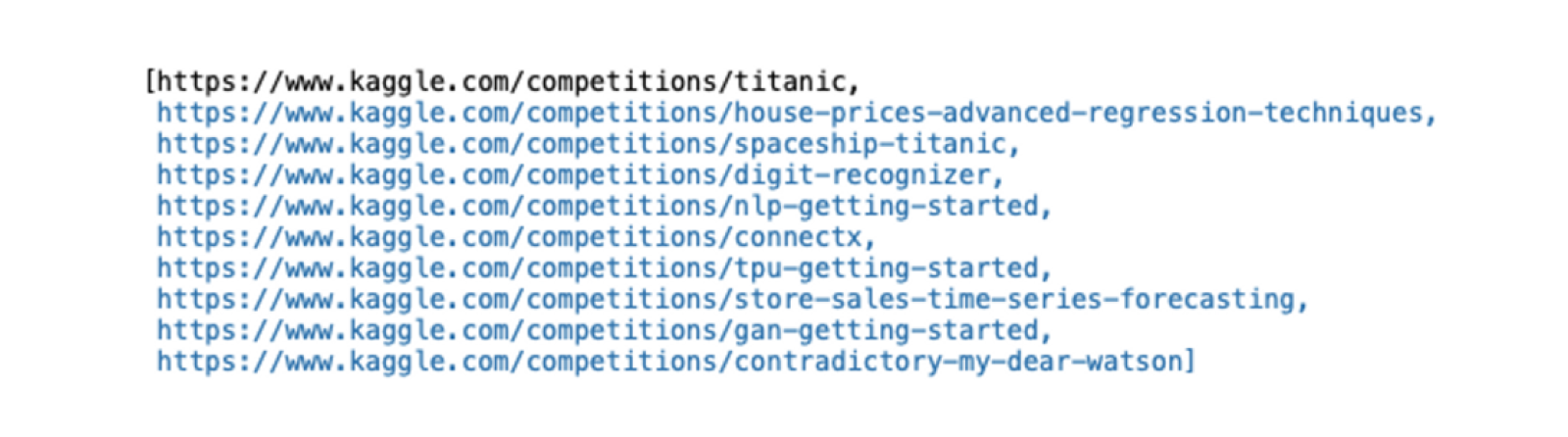

Competition List

If you want to access the data from a specific competition, just provide the name of the competition in the competition_list_files() function.

# choose a specific competition
api.competition_download_files('titanic')

To download the files for this competition, you can use the competition_download_files() method and provide the competition name as an argument.

# list data of a competition
api.competition_download_files('titanic')

Now you have the dataset to work with.

Accessing financial data using pandas_datareader

If you need specific financial and economic data, pandas_datareader pulls data Yahoo Finance, Google Finance, Federal Reserve Economic Data (FRED), and World Bank. It is an extension to the most popular pandas library and simplifies the process of accessing time series data like stock prices, economic indicators, and more.

You can download the dependency using PIP as follows:

$ pip install pandas_datareader

Once downloaded, you can use the following code to access the Gold stock price from Yahoo as follows:

# import dependency
from pandas_datareader import dataimport datetime as dt

# access gold price between 2019-01-01 to today
zm = data.get_data_yahoo(
	"GOLD",
	start='2019-1-1',
	end=dt.datetime.today()).reset_index()

# show the first few rows of data
zm.head()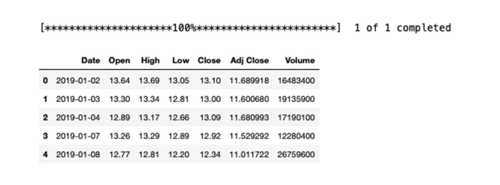

You can find the notebook and datasets used for this tutorial here.

Access any data with Python and Jupyter

Python and Jupyter streamlines the process of sourcing and analyzing data. With the plethora of libraries and tools available, accessing diverse datasets is incredibly easy. Whether you're pulling financial data, querying databases, or leveraging platforms like Kaggle, the combined power of Python and Jupyter ensures a better experience for accessing data for analysts.

Want to learn more about Jupyter notebooks?

Here are some of our other articles:

Want to supercharge your Jupyter notebooks? Try Hex! Hex is a powerful notebook UI that lets you analyze data in SQL, Python, or no-code, in any combination. With Hex, you can work together with live multiplayer and version control, and easily share your insights with beautiful reports and dashboards — all built in.

✨ Get started for free

🕵️ Learn more