Customer Segmentation

You can’t hand out a unique discount to every single customer or design a one-off strategy for each individual. This is impossible, especially in B2C businesses like e-commerce and banking.

Instead, companies group similar customers and make decisions at the segment level. By clustering people with shared behaviors or traits, you can roll out personalized experiences and targeted strategies without drowning in complexity at the individual level.

In this blog, we’ll walk through the steps to implement customer segmentation and explore the tools that help you segment effectively. 

What is Customer Segmentation?

Customer segmentation is the process of dividing a customer base into groups that share similar needs, behaviors, or characteristics.

B2C businesses' customer segments are generally based on factors such as demographics, lifestyle, values, and needs. B2B marketers segment customers by industry, location, or contract durations.

Tools like Hex and Python make this process much easier. With techniques such as K-Means clustering, you can group customers based on behavior, demographics, or other signals. From there, those segments can drive targeted marketing campaigns or fuel personalized product experiences.

We’ll walk through exactly how to do this. But first, let’s zoom in on why customer segmentation matters in the first place.

Why Customer Segmentation Matters

No customer is the same. They all have their little quirks. Some like personalized attention, while others prefer a more hands-off approach. Some are price-sensitive, always looking for the best deal, while others prioritize quality and are willing to pay a premium for superior products or services. Some customers are loyal to a brand, while others are more fickle and easily swayed by the latest trends or promotions.

To cater to this diverse range of preferences, businesses often employ customer segmentation. Once you understand the attributes of each segment, you can tailor marketing strategies, product offerings, and customer experiences to fit those groups more effectively.

Marketers often create buyer personas for each major segment to capture what makes those customers tick. They study the behaviors and motivations of each group, then craft brand messaging and positioning that resonate. 

When a new user joins, the business maps them to the closest segment and applies the same playbook, delivering a service that feels more personal.

Additionally, by analyzing what each customer group values, companies can identify which products or services to invest in next and spot ways to improve retention. This leads to a smarter, more focused approach to growth.

Types of Customer Segmentation

There are four core ways to segment customers:

Demographic Segmentation

Demographic segmentation involves dividing customers based on demographic variables such as age, gender, income, education level, marital status, or occupation. This type of segmentation is relatively easy to implement since demographic data is often readily available.

For example, a clothing retailer might segment its customers based on age and gender to offer targeted product lines and marketing campaigns. A luxury car manufacturer might focus on high-income individuals, while a budget-friendly grocery store might target families with lower incomes.

Geographic Segmentation

Geographic segmentation divides customers based on their geographic location, such as country, state, city, or even neighborhood. This type of segmentation is beneficial for businesses that operate in multiple regions or have products or services that vary based on location.

For instance, a restaurant chain might offer different cuisines or promotions based on the local preferences and tastes of each region. A global e-commerce company might segment its customers based on country to provide localized website content, payment options, and shipping methods.

Psychographic Segmentation

Psychographic segmentation groups customers based on their personality traits, values, attitudes, interests, and lifestyles. This type of segmentation goes beyond demographic factors and focuses on the psychological aspects that influence customer behavior.

For example, a travel company might segment its customers based on their travel preferences, such as adventure seekers, luxury travelers, or budget-conscious backpackers. A health food store might target customers who value organic and natural products, while a tech company might focus on early adopters and tech enthusiasts.

Behavioral Segmentation

Behavioral segmentation categorizes customers based on their actions and interactions with a brand, including purchase history, website browsing behavior, brand loyalty, and usage frequency. This type of segmentation focuses on how customers behave and engage with a company's products or services.

For example, an e-commerce company might segment its customers based on their purchase frequency and average order value to offer personalized recommendations and loyalty rewards. A subscription-based service segment customers based on their usage patterns and engagement levels to prevent churn and improve retention.

By understanding these different types of customer segmentation, businesses can choose the most appropriate approach or combination of approaches to effectively segment their customer base and deliver targeted experiences that resonate with each segment.

Key Elements of an Effective Customer Segmentation Strategy

Clear Objectives

Every segmentation strategy should start with clear goals. Whether it’s reducing churn, increasing sales, or tailoring marketing campaigns, defining objectives upfront ensures that segmentation efforts are aligned with business outcomes. 

Clear goals also guide which segmentation model to use. For instance, if your objective is expansion into new markets, geographic segmentation will help you localize campaigns and speak directly to regional audiences. If your goal is to retain existing customers, behavioral segmentation might be the smarter choice.

Relevant Data Usage

Effective customer market segmentation relies on robust data collection and analytics. Businesses might collect comprehensive customer data from surveys, website or product interactions, and social media for future analysis.

But while building a segmentation model, it’s important to focus only on the relevant data. 

This becomes much easier if you already know the type of segmentation you’re aiming for. For demographic segmentation, you’ll need age, gender, and income details. For behavioral segmentation, focus on metrics like purchase frequency and product usage. By pulling only the required data into your Notebooks, you reduce preprocessing efforts and keep models more focused. 

Data Quality

Once the data is collected, the next critical step is ensuring quality. Customers sometimes fill out forms with incomplete or even false information, leaving gaps in your dataset. Regional differences, like date formats, also create inconsistencies. And when data is spread across multiple sources like emails, surveys, and support tickets, duplicate entries often appear during consolidation.

Addressing these issues is essential for creating a reliable dataset. Without this step, even the most advanced segmentation model can be ineffective.

Meaningful Segments

Segments should be both large enough to be actionable and clearly distinct from each other. Only focusing on these segments will drive the actual growth.

For example, if you segment the data by age and the “children” group is very sparse, it may not be worthwhile to invest significant resources in targeted campaigns for that group. 

Also, ensure each segment is distinct from the others, since only then does it make sense to create tailored campaigns for each one.

Steps to Implement Customer Segmentation

Let’s walk through an example of customer segmentation. Here, we’re going to use hex and Python to build clusters for our existing customers, and predict which cluster a new customer will fit into depending on their features.

First, let’s import the libraries we’ll need:

import pandas as pd
import numpy as np
import matplotlib.pyplot as plt
from sklearn.cluster import KMeans, AgglomerativeClustering
from sklearn.metrics.pairwise import cosine_similarity
from sklearn.preprocessing import StandardScaler, LabelEncoder
from sklearn.decomposition import PCA, SparsePCA

import plotly.graph_objects as go

We use `pandas` for data manipulation and analysis, with data structures like `DataFrames` and `Series`, and `numpy` for numerical computing.

For visualization, we rely on two libraries. That is, `matplotlib.pyplot` to create static, animated, and interactive plots. Then, `plotly.graph_objects` from the Plotly library to build interactive, publication-quality visualizations.

However, the core libraries for clustering are provided by sklearn. These are:

• `sklearn.cluster`: Implements clustering algorithms such as K-Means and Agglomerative Clustering.
• `sklearn.metrics.pairwise`: Computes pairwise distances or similarities between samples, including cosine similarity.
• `sklearn.preprocessing`: Includes data preprocessing utilities, such as scaling, normalization, and encoding.
• `sklearn.decomposition`: Performs dimensionality reduction with techniques like Principal Component Analysis (PCA) and Sparse PCA.

Data Querying

Once we import the modules, we load the data. We use a sample e-commerce dataset for this example. With Hex Notebooks, we can run Python and SQL side by side, so we query the dataset directly from the data warehouse using SQL:

SELECT
    u.USER_ID,
    u.AGE,
    u.GENDER,
    u.COUNTRY,
    u.TRAFFIC_SOURCE,
    COUNT(o.ORDER_ID) AS total_orders,
    ii_most_common_brand.PRODUCT_BRAND AS most_frequent_brand,
    ii_most_common_category.PRODUCT_CATEGORY AS most_frequent_category
FROM DEMO_DATA.ECOMMERCE.USERS AS u
LEFT JOIN DEMO_DATA.ECOMMERCE.ORDERS AS o ON u.USER_ID = o.USER_ID
LEFT JOIN DEMO_DATA.ECOMMERCE.ORDER_ITEMS AS oi ON oi.ORDER_ID = o.ORDER_ID
LEFT JOIN DEMO_DATA.ECOMMERCE.INVENTORY_ITEMS as ii ON oi.INVENTORY_ITEM_ID = ii.ID
LEFT JOIN (
    SELECT
        USER_ID,
        PRODUCT_BRAND,
        ROW_NUMBER() OVER (PARTITION BY USER_ID ORDER BY COUNT(*) DESC) AS brand_rank
    FROM DEMO_DATA.ECOMMERCE.ORDER_ITEMS AS oi
    JOIN DEMO_DATA.ECOMMERCE.INVENTORY_ITEMS as ii ON oi.INVENTORY_ITEM_ID = ii.ID
    GROUP BY USER_ID, PRODUCT_BRAND
) AS ii_most_common_brand ON ii_most_common_brand.USER_ID = u.USER_ID AND ii_most_common_brand.brand_rank = 1
LEFT JOIN (
    SELECT
        USER_ID,
        PRODUCT_CATEGORY,
        ROW_NUMBER() OVER (PARTITION BY USER_ID ORDER BY COUNT(*) DESC) AS category_rank
    FROM DEMO_DATA.ECOMMERCE.ORDER_ITEMS AS oi
    JOIN DEMO_DATA.ECOMMERCE.INVENTORY_ITEMS as ii ON oi.INVENTORY_ITEM_ID = ii.ID
    GROUP BY USER_ID, PRODUCT_CATEGORY
) AS ii_most_common_category ON ii_most_common_category.USER_ID = u.USER_ID AND ii_most_common_category.category_rank = 1
GROUP BY
    u.USER_ID,
    u.AGE,
    u.GENDER,
    u.COUNTRY,
    u.TRAFFIC_SOURCE,
    ii_most_common_brand.PRODUCT_BRAND,
    ii_most_common_category.PRODUCT_CATEGORY
HAVING total_orders > 0

This is a big query, but basically it joins multiple tables to retrieve user information, total orders, the most frequently purchased product brand, and the most commonly purchased product category for each user who has placed at least one order.

The end result is a comprehensive view of each user's profile, including their demographic information, total orders, and the brand and category they most frequently purchase from. 

This information can be valuable for customer segmentation, targeted marketing campaigns, and understanding user preferences in an e-commerce setting.

Preprocessing

Then we run through some basic preprocessing. First, we copy the data:

original_data = data.copy()

Then we remove any missing values:

data = data.dropna()

Then, we’ll print out a summary of the data to better understand it:

data.info()

<class 'pandas.core.frame.DataFrame'>
RangeIndex: 80061 entries, 0 to 80060
Data columns (total 8 columns):
 #   Column                  Non-Null Count  Dtype 
---  ------                  --------------  ----- 
 0   USER_ID                 80061 non-null  int64 
 1   AGE                     80061 non-null  int64 
 2   GENDER                  80061 non-null  object
 3   COUNTRY                 80061 non-null  object
 4   TRAFFIC_SOURCE          80061 non-null  object
 5   TOTAL_ORDERS            80061 non-null  int64 
 6   MOST_FREQUENT_BRAND     80061 non-null  object
 7   MOST_FREQUENT_CATEGORY  80061 non-null  object
dtypes: int64(3), object(5)
memory usage: 4.9+ MB

We then want to use `sklearn` for some cluster-specific data prep:

from sklearn.preprocessing import LabelEncoder

# Initialize a LabelEncoder object
encoder = LabelEncoder()

# Encode categorical variables
data["GENDER"] = encoder.fit_transform(data["GENDER"])
data["COUNTRY"] = encoder.fit_transform(data["COUNTRY"])
data["TRAFFIC_SOURCE"] = encoder.fit_transform(data["TRAFFIC_SOURCE"])
data["MOST_FREQUENT_BRAND"] = encoder.fit_transform(data["MOST_FREQUENT_BRAND"])
data["MOST_FREQUENT_CATEGORY"] = encoder.fit_transform(data["MOST_FREQUENT_CATEGORY"])

# Check the transformed data
data.head()

The LabelEncoder assigns a unique numerical label to each category in a variable. For example, if the `GENDER` variable has categories "Male" and "Female", the encoder might assign the label 0 to "Male" and 1 to "Female". This transformation represents categorical data numerically, making it suitable for machine learning algorithms that require numerical inputs.

Keep in mind that LabelEncoder assigns labels arbitrarily and does not capture any ordinal relationship between categories. When the data has an inherent order or hierarchy, techniques like OrdinalEncoder or custom mappings work better.

Dimensionality Reduction

At this point, we can start with a critical part of clustering: dimensionality reduction. 

In high-dimensional datasets with many features, clustering algorithms often struggle to find meaningful patterns because of the curse of dimensionality.

So, dimensionality reduction simplifies the data by reducing the number of features or variables while retaining the most important information. 

reducer = PCA(n_components = 2, random_state = 444)
scaler = StandardScaler()

# run PCA on the scaled features and create a dataframe from the components
features = scaler.fit_transform(data)
reduced_features = reducer.fit_transform(features) 
components = pd.DataFrame(reduced_features, columns = ['component_1', 'component_2'])

This code performs Principal Component Analysis (PCA) on the dataset to reduce its dimensionality and create a new DataFrame with the transformed components. 

PCA is a technique used for dimensionality reduction and feature extraction. It identifies the principal components that capture the most variance in the dataset.

Here's a breakdown of the code:

• We initialize the PCA object with `n_components` = 2 and `random_state `= 444. This means that PCA will reduce the dataset to two principal components, and the random state is set to 444 for reproducibility.
• We create a `StandardScaler` object to standardize the features before applying PCA. Standardization matters because PCA is sensitive to feature scale. After scaling, each feature has a mean of 0 and a standard deviation of 1.
• We apply the `fit_transform()` method of the scaler to the dataset (`data`) and store the scaled features in the features variable.
• We then apply the `fit_transform()` method of the PCA object to the scaled features (`features`). This step performs dimensionality reduction and transforms the dataset into a lower-dimensional space. We store the result in the reduced_features variable.
• Finally, we create a new DataFrame called `components` from the transformed data (`reduced_features`). We label the columns `component_1` and `component_2`, representing the two principal components.

By reducing the dimensionality to two components, PCA helps to visualize and understand the underlying structure of the data in a lower-dimensional space.

The resulting `components` DataFrame contains the transformed data points in the reduced two-dimensional space. Each row represents a data point, and the columns ('component_1' and 'component_2') represent the values of the two principal components for that data point. This transformed dataset can be used for further analysis, visualization, or as input to other machine learning algorithms.

Clustering and Segmentation

Then we can perform the actual clustering and segmentation:

from sklearn.cluster import KMeans

# Define a function to calculate the clustering score for a given number of clusters
def get_kmeans_score(data, center):
    kmeans = KMeans(n_clusters=center)
    model = kmeans.fit(data)
    score = model.score(data)
    return abs(score)

# Determine the range of number of clusters
centers = list(range(2, 11))

# Calculate the clustering score for each number of clusters
scores = [get_kmeans_score(components, center) for center in centers]

The code defines a function called `get_kmeans_score()` that takes two parameters: data (the input dataset) and center (the number of clusters to use).

Inside the function, we initialize a KMeans object with the specified number of clusters using `KMeans(n_clusters=center)`. We then call the `fit()` method on the KMeans object and pass in the input data (`data`). This step trains the K-Means model on the dataset and identifies the optimal cluster centers.

Next, we call the `score()` method on the trained model, again passing the input data (data). This calculates the clustering score, which measures how well the data points fit into their assigned clusters. The score is usually the negative sum of squared distances between each data point and its nearest cluster center.

The absolute value of the score is returned using `abs(score)`. Taking the absolute value ensures that the score is positive.

We then use this function to calculate the clustering score for each number of clusters in the `centers` list. By calculating the clustering score for different numbers of clusters, this code helps determine the optimal number of clusters for the given dataset. 

The optimal number of clusters is often chosen based on the elbow method, where the number of clusters is selected at the point where the rate of decrease in the clustering score slows down significantly.

We can then plot these scores:

plt.figure(figsize=(10, 6))
plt.plot(centers, scores, linestyle='--', marker='o', color='b')
plt.xlabel('K')
plt.ylabel('SSE')
plt.title('SSE vs. K')
plt.show()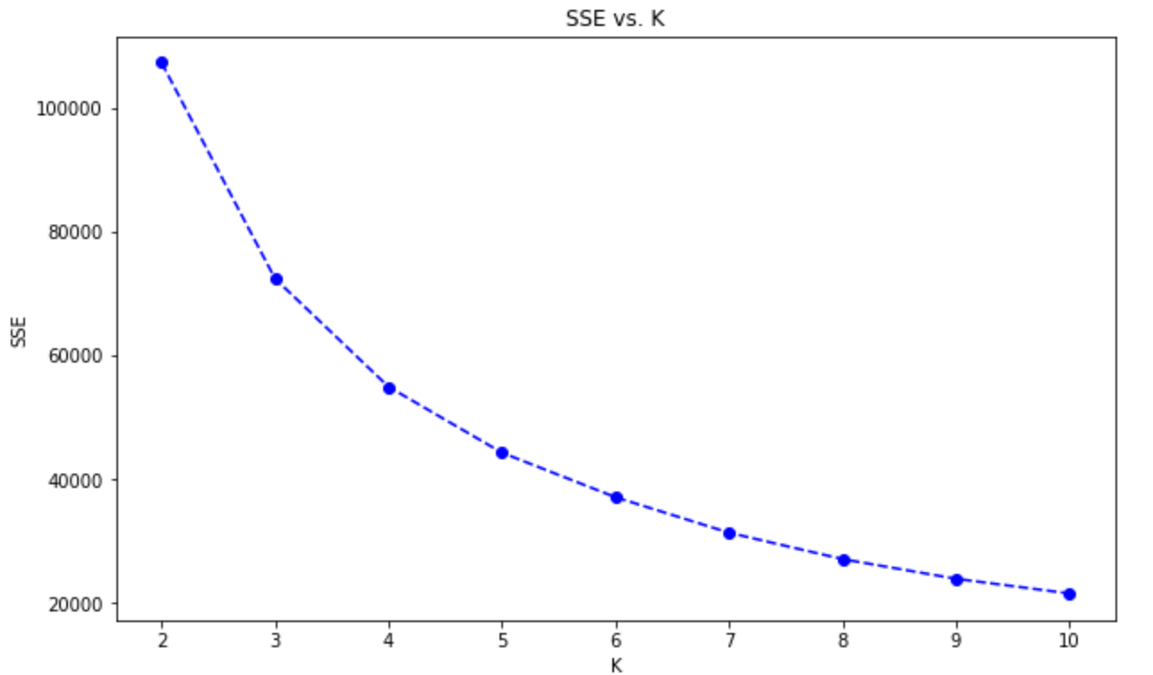

We see an "Elbow" at ~5 clusters, which means it doesn't get meaningfully better after that. We'll use five as our number of clusters in our K-Means.

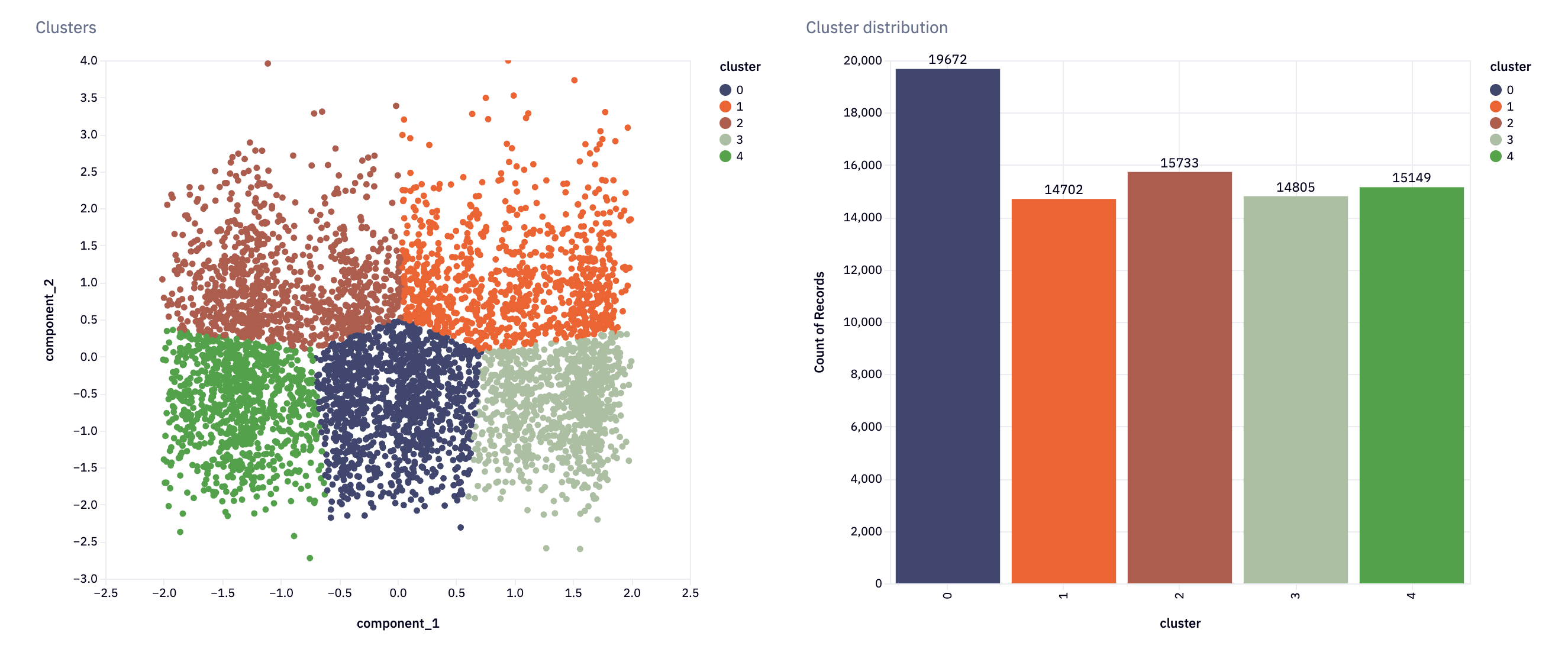
kmeans = KMeans(n_clusters=5, init='k-means++', max_iter=300, n_init=10, random_state=222) kmeans.fit(components) components['cluster'] = kmeans.labels_ dataset = pd.concat([data, components], axis = 1)

This performs the actual K-means clustering on our dataset. It initializes a `KMeans` object with specified parameters, fits the model to the input data, assigns the resulting cluster labels to each data point, and concatenates the original data with the cluster assignments and component values obtained from dimensionality reduction.

After executing this code, the dataset dataframe will contain the original data columns, the cluster assignments, and the component values. Each data point will have a corresponding cluster label, indicating which cluster it belongs to based on the K-means clustering algorithm.

This code is commonly used in the context of customer segmentation or grouping similar data points based on their features. By assigning cluster labels to each data point, it becomes easier to analyze and understand the underlying structure and patterns in the data. The resulting dataset can be further analyzed, visualized, or used for downstream tasks such as targeted marketing, personalized recommendations, or customer profiling.

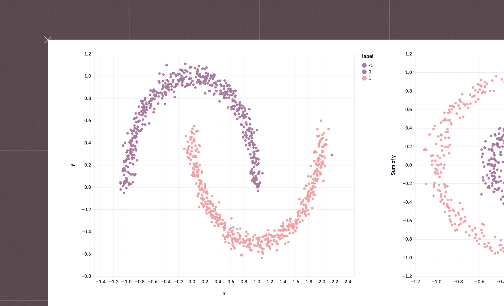
We can, in fact, visualize this data with Hex’s in-built charting:

Visualizations are helpful, but analysts also like to see the raw numbers and summary statistics. To do that, we’ll build a report for each cluster:

columns_to_report = ['AGE', 'GENDER', 'TOTAL_ORDERS', 'TRAFFIC_SOURCE','MOST_FREQUENT_BRAND','MOST_FREQUENT_CATEGORY']

def build_report(cluster):
    report = {}
    for col in columns_to_report:
        group = dataset[dataset['cluster'] == cluster]
        info = group.groupby(col)[['USER_ID']].count().sort_values(by = 'USER_ID', ascending = False).reset_index()
        info['ratio'] = np.round((info['USER_ID'] / info['USER_ID'].sum()) * 100, 2)
        top_5 = info[[col, 'ratio']].iloc[:3].values
        report[col] = top_5
        report['cluster_ratio'] = np.round((group.shape[0] / dataset.shape[0]) * 100, 2)
    return report

report1 = build_report(0)
report2 = build_report(1)
report3 = build_report(2)
report4 = build_report(3)
report5 = build_report(4)

`build_report()` generates a report for each cluster in a dataset.

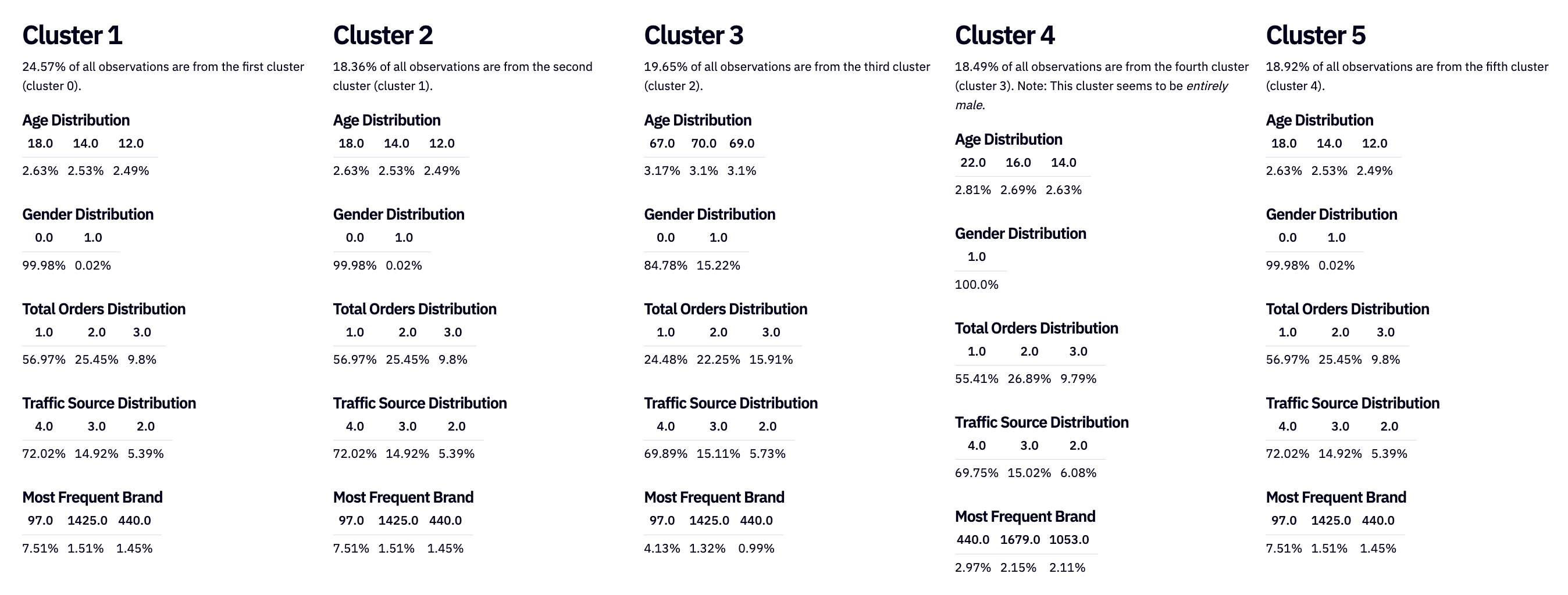
You can use the reports to gain insights into the characteristics and patterns of the data points within each cluster. These insights help you understand how customers or data points are segmented based on the chosen columns.

Predicting Customer Segmentation

With our current customers clustered, we can now use that information to try to predict segments for new customers. This approach lets us quickly and accurately assign new customers to the most appropriate segment based on their characteristics, behaviors, or preferences. By leveraging insights from the existing customer base, we streamline how we understand and target new customers.

features = [{
    "AGE": age,
    "GENDER": gender,
    "COUNTRY": country,
    "TOTAL_ORDERS": total_orders,
    "TRAFFIC_SOURCE": traffic_source,
    "MOST_FREQUENT_BRAND": favorite_brand,
    "MOST_FREQUENT_CATEGORY": favorite_category,
}]
user = pd.DataFrame(features)
encoder = LabelEncoder()

# Encode categorical variables
user["GENDER"] = encoder.fit_transform(user["GENDER"])
user["COUNTRY"] = encoder.fit_transform(user["COUNTRY"])
user["TRAFFIC_SOURCE"] = encoder.fit_transform(user["TRAFFIC_SOURCE"])
user["MOST_FREQUENT_BRAND"] = encoder.fit_transform(user["MOST_FREQUENT_BRAND"])
user["MOST_FREQUENT_CATEGORY"] = encoder.fit_transform(user["MOST_FREQUENT_CATEGORY"])

The purpose of this code is to prepare the new user profile data for further analysis or prediction. By encoding categorical variables as numerical values, we make the data compatible with machine learning algorithms that require numerical inputs.

We can then use it to make predictions:

if make_prediction:
    user_data = {}
    # loop through all the columns present in the original encoded dataframe
    for column in data.columns:
        # if the column is already present in the `user` dictionary (from code cell 40)
        if column in user_dict:
            # then add the data to the user_data dictionary
            user_data[column] = user_dict[column]
        # if the column is not in the dataframe
        else:
            # add the column to the dataframe and set the value to 0 (since it's not present)
            user_data[column] = 0

# create an updated user_data dataframe
user_data = pd.DataFrame([user_data])

    # transform features into components
    scaled_user_data = scaler.transform(user_data)
    user_components = reducer.transform(scaled_user_data)
    component_df = pd.DataFrame(user_components, columns = ['component_1', 'component_2'])

    # predict cluster
    cluster = kmeans.predict(component_df)
    component_df['cluster'] = cluster
    user_df = pd.concat([user_data, component_df], axis = 1)

    # find similar users
    df1 =  user_df
    df2 =  dataset

    similarity = cosine_similarity(user_df[['component_1', 'component_2']], dataset[['component_1', 'component_2']])
    dataset['similarity_score'] = similarity[0] * 100
    top5 = df2.sort_values(by = 'similarity_score', ascending = False).iloc[:5] #.to_dict(orient = 'records')
else:
    user_data = None
    cluster = None
    user_df = pd.DataFrame()
    top5 = pd.DataFrame()

This code takes a user’s data, transforms it into components using the same scaling and dimensionality reduction techniques applied to the original dataset, predicts the user’s cluster, and then finds the top five most similar users based on the cosine similarity of their components.

• We apply the `scaler.transform()` method to `user_data` to scale the features.
• We apply the `reducer.transform()` method to the scaled data to reduce dimensionality and obtain the user’s components.
• We store the resulting components in a DataFrame called `component_df` with the columns `component_1` and `component_2`.

The `kmeans.predict()` method is used to predict the cluster to which the user belongs based on their components. The predicted cluster is added as a new column 'cluster' to the `component_df`.

The `user_data` and `component_df` DataFrames are concatenated along the column axis to create a new DataFrame called `user_df`, which contains both the user's data and their components.

The code then finds similar users to the given user:

• We calculate the cosine similarity between the user’s components and the components of all users in the dataset using `cosine_similarity()`.
• We then add the similarity scores as a new column called `similarity_score` in the dataset DataFrame.
• We sort the DataFrame by similarity scores, select the top five users with `sort_values()` and `iloc[]`, and store the result in `top5`.

The resulting `user_df` DataFrame contains the user's data along with their components and predicted cluster, while the `top5` DataFrame contains the top five most similar users to the given user.

Tools for Customer Segmentation

To segment customers effectively, you need the right tools at every stage: collecting, storing, and analyzing data for valuable insights. Let's look at the important ones:

Data Collection Tools

Data collection tools integrate with multiple sources, including websites, surveys, support tickets, email systems, payment platforms, and more, to consolidate raw customer data into a single location.

CRMs and customer data platforms, such as ContentSquare, HubSpot, or Twilio, are common choices. They work by embedding SDKs or APIs into your source systems to capture interaction data in real time. Some tools even map these data points into a single customer profile before loading them into your warehouse. 

Data Warehouse

Once collected, all that customer data is loaded to a central repository, like a data warehouse. Cloud solutions like Snowflake, Databricks, and Redshift are the go-to warehouses that can handle large volumes of structured data at scale.

With everything in one place, teams can easily pull data for analytics, reporting, or modeling. 

Data Analytics Platforms

Analytics platforms sit on top of the warehouse and let you actually perform customer segmentation. At a basic level, you can create simple segments with BI tools by filtering on characteristics like location or purchase frequency, then visualize them in reports.

But when you want to capture real behavioral patterns, you’ll need machine learning techniques. Tools like Hex connect seamlessly to your warehouse and provide access to updated data in Jupyter-like Notebooks. Within the same Notebook, you can write SQL, Python, or R to model customer behavior. Once the model is ready, you can build dynamic dashboards that showcase results to stakeholders.

Business users can interact with these dashboards directly, adjusting inputs and extracting the insights they need.

Challenges in Customer Segmentation

Data Silos

Customer data is often found across multiple systems — CRMs, support platforms, payment systems, and marketing tools. 

Without strong integrations between these platforms, the data remains fragmented, leading to incomplete or inconsistent customer profiles. So, breaking down these data silos and unifying data streams can be challenging in more scattered environments.

Technical Capabilities

Not every segmentation need can be met with simple BI dashboards. Sometimes you need deeper insights, like identifying hidden behavioral patterns, which calls for machine learning models. But building and maintaining those models requires technical expertise. You’ll need data scientists or analysts who can train models, validate results, and then serve insights to stakeholders in a way that’s easy to understand, often through intuitive dashboards. Without this expertise, businesses risk oversimplifying segmentation or failing to scale it.

Changing Demands

Segmentation is not a one-and-done project. Customer behavior evolves, business goals shift, and markets change over time. Your segmentation framework needs to adapt to them. And this is one of the tricky challenges in customer segmentation. 

To address this, build flexibility into your systems from the start. Use adaptable schemas during data collection so pipelines don’t break when input formats change. Set up alerts to flag drops in model accuracy. And design processes that can incorporate new data flows seamlessly, ensuring your segmentation stays adaptable and scalable over time.

Conclusion

Customer segmentation using Python and tools like Hex empowers businesses to unlock the full potential of their customer data. By leveraging advanced clustering techniques, such as K-Means, businesses can gain deep insights into their customers, make data-driven decisions, and create targeted strategies that drive customer satisfaction and business success.

To build your customer segmentation models more efficiently, sign up for Hex today!