Customer Segmentation

Izzy Miller
Enhance your marketing and sales strategies with a detailed Customer Segmentation model built using SQL & Python. Using K-Means clustering, you can intelligently segment ...
How to build: Customer Segmentation
No customer is the same. They all have their little quirks. Some like personalized attention, while others prefer a more hands-off approach. Some are price-sensitive, always looking for the best deal, while others prioritize quality and are willing to pay a premium for superior products or services. There are customers who are loyal to a brand, and those who are more fickle, easily swayed by the latest trends or promotions.
To effectively cater to these diverse preferences and behaviors, businesses often engage in customer segmentation. This process involves dividing a customer base into distinct groups that share similar characteristics, needs, or desires. By understanding the unique attributes of each segment, companies can tailor their marketing strategies, product offerings, and customer service to better meet the expectations of each group.
With Hex and Python, you can use K-Means clustering to segment your customers into different groups based on their behavior, demographics, or other characteristics. You can then use these customer segments in your marketing campaigns or within your product for personalized experiences.
We are going to walk through how to do so, but first let’s take a closer look at customer segmentation.
The 4 Types of Customer Segmentation
There are four core ways to segment customers:
Demographic segmentation
Demographic segmentation involves dividing customers based on demographic variables such as age, gender, income, education level, marital status, or occupation. This type of segmentation is relatively easy to implement since demographic data is often readily available and can provide valuable insights into customer preferences and behaviors.
For example, a clothing retailer might segment their customers based on age and gender to offer targeted product lines and marketing campaigns. A luxury car manufacturer might focus on high-income individuals, while a budget-friendly grocery store might target families with lower incomes.
Geographic segmentation
Geographic segmentation divides customers based on their geographic location, such as country, state, city, or even neighborhood. This type of segmentation is particularly useful for businesses that operate in multiple regions or have products or services that vary based on location.
For instance, a restaurant chain might offer different menu items or promotions based on the local preferences and tastes of each region. A global e-commerce company might segment their customers based on country to provide localized website content, payment options, and shipping methods.
Psychographic segmentation
Psychographic segmentation groups customers based on their personality traits, values, attitudes, interests, and lifestyles. This type of segmentation goes beyond demographic factors and focuses on the psychological aspects that influence customer behavior.
For example, a travel company might segment their customers based on their travel preferences, such as adventure seekers, luxury travelers, or budget-conscious backpackers. A health food store might target customers who value organic and natural products, while a tech company might focus on early adopters and tech enthusiasts.
Behavioral segmentation
Behavioral segmentation divides customers based on their actions and interactions with a brand, such as purchase history, website browsing behavior, brand loyalty, or usage frequency. This type of segmentation focuses on how customers behave and engage with a company's products or services.
For example, an e-commerce company might segment their customers based on their purchase frequency and average order value to offer personalized recommendations and loyalty rewards. A subscription-based service might segment customers based on their usage patterns and engagement levels to prevent churn and improve retention.
By understanding these different types of customer segmentation, businesses can choose the most appropriate approach or combination of approaches to effectively segment their customer base and deliver targeted experiences that resonate with each segment.
The Benefits of Customer Segmentation
Customer segmentation offers numerous benefits to businesses by enabling them to better understand and serve their customers. Some of the key advantages include:
Targeted Marketing: By segmenting customers into distinct groups, businesses can develop targeted marketing campaigns that resonate with each segment's specific needs, preferences, and behaviors. This personalized approach leads to higher engagement, better conversion rates, and increased customer loyalty.
Improved Product Development: Understanding the unique requirements and preferences of different customer segments allows companies to develop products or services that cater to specific segments. This targeted approach ensures that product offerings align with customer needs, resulting in higher satisfaction and adoption rates.
Enhanced Customer Service: Segmentation enables businesses to tailor their customer service strategies to meet the expectations of each segment. By understanding the communication preferences, support needs, and pain points of different segments, companies can deliver personalized and efficient customer service, leading to increased customer satisfaction and retention.
Optimized Resource Allocation: Customer segmentation helps businesses allocate their resources more effectively. By focusing on the most valuable or promising segments, companies can prioritize their efforts and investments, ensuring that resources are directed towards initiatives that yield the highest returns.
Competitive Advantage: By deeply understanding their customer segments, businesses can identify untapped opportunities, anticipate market trends, and differentiate themselves from competitors. This customer-centric approach allows companies to stay ahead of the curve and gain a competitive edge in their industry.
Increased Customer Lifetime Value: Segmentation enables businesses to identify and nurture high-value customer segments. By providing personalized experiences, cross-selling relevant products, and implementing loyalty programs, companies can increase customer lifetime value and foster long-term relationships with their most profitable customers.
Data-Driven Decision Making: Customer segmentation is based on data analysis, allowing businesses to make informed decisions based on real customer insights. By leveraging data-driven segmentation, companies can minimize guesswork and rely on evidence-based strategies to drive growth and profitability.
By leveraging customer segmentation, businesses can allocate their resources more efficiently, improve customer satisfaction, and ultimately drive growth and profitability. However, it's essential to remember that while segmentation is a powerful tool, customers are still individuals with unique needs and preferences that may not always fit neatly into predefined categories.
Using Hex and Python for Customer Segmentation
Let’s walk through an example of customer segmentation. Here, we’re going to use hex and Python to build clusters for our existing customers, and predict which cluster a new customer will fit into depending on their features.
First, let’s import the libraries we’ll need:
import pandas as pd
import numpy as np
import matplotlib.pyplot as plt
from sklearn.cluster import KMeans, AgglomerativeClustering
from sklearn.metrics.pairwise import cosine_similarity
from sklearn.preprocessing import StandardScaler, LabelEncoder
from sklearn.decomposition import PCA, SparsePCA

import plotly.graph_objects as go
We're using pandas for data manipulation and analysis, providing data structures like DataFrames and Series and numpy for numerical computing.
You’ll see where’re going to do some plotting further down. For that we’re going to use matplotlib.pyplot for creating static, animated, and interactive visualizations and then plotly.graph_objects from the Plotly library that allows the creation of interactive and publication-quality visualizations.
But the core libraries for clustering come from sklearn. These are:
sklearn.cluster: A module from the scikit-learn library that provides implementations of clustering algorithms like K-Means and Agglomerative Clustering.sklearn.metrics.pairwise: A module that offers functions for computing pairwise distances or similarities between sets of samples, such as cosine similarity.sklearn.preprocessing: A module that provides various data preprocessing utilities, including scaling, normalization, and encoding.sklearn.decomposition: A module that offers dimensionality reduction techniques like Principal Component Analysis (PCA) and Sparse PCA.
Data Querying
Once we have our modules, then we can get our data. We’re using a sample ecommerce dataset. In Hex, we can use Python and SQL side-by-side, so we’ll query our data from our data warehouse directly using SQL:
SELECT
    u.USER_ID,
    u.AGE,
    u.GENDER,
    u.COUNTRY,
    u.TRAFFIC_SOURCE,
    COUNT(o.ORDER_ID) AS total_orders,
    ii_most_common_brand.PRODUCT_BRAND AS most_frequent_brand,
    ii_most_common_category.PRODUCT_CATEGORY AS most_frequent_category
FROM DEMO_DATA.ECOMMERCE.USERS AS u
LEFT JOIN DEMO_DATA.ECOMMERCE.ORDERS AS o ON u.USER_ID = o.USER_ID
LEFT JOIN DEMO_DATA.ECOMMERCE.ORDER_ITEMS AS oi ON oi.ORDER_ID = o.ORDER_ID
LEFT JOIN DEMO_DATA.ECOMMERCE.INVENTORY_ITEMS as ii ON oi.INVENTORY_ITEM_ID = ii.ID
LEFT JOIN (
    SELECT
        USER_ID,
        PRODUCT_BRAND,
        ROW_NUMBER() OVER (PARTITION BY USER_ID ORDER BY COUNT(*) DESC) AS brand_rank
    FROM DEMO_DATA.ECOMMERCE.ORDER_ITEMS AS oi
    JOIN DEMO_DATA.ECOMMERCE.INVENTORY_ITEMS as ii ON oi.INVENTORY_ITEM_ID = ii.ID
    GROUP BY USER_ID, PRODUCT_BRAND
) AS ii_most_common_brand ON ii_most_common_brand.USER_ID = u.USER_ID AND ii_most_common_brand.brand_rank = 1
LEFT JOIN (
    SELECT
        USER_ID,
        PRODUCT_CATEGORY,
        ROW_NUMBER() OVER (PARTITION BY USER_ID ORDER BY COUNT(*) DESC) AS category_rank
    FROM DEMO_DATA.ECOMMERCE.ORDER_ITEMS AS oi
    JOIN DEMO_DATA.ECOMMERCE.INVENTORY_ITEMS as ii ON oi.INVENTORY_ITEM_ID = ii.ID
    GROUP BY USER_ID, PRODUCT_CATEGORY
) AS ii_most_common_category ON ii_most_common_category.USER_ID = u.USER_ID AND ii_most_common_category.category_rank = 1
GROUP BY
    u.USER_ID,
    u.AGE,
    u.GENDER,
    u.COUNTRY,
    u.TRAFFIC_SOURCE,
    ii_most_common_brand.PRODUCT_BRAND,
    ii_most_common_category.PRODUCT_CATEGORY
HAVING total_orders > 0
This is a big query, but basically it joins multiple tables to retrieve user information, total orders, most frequently purchased product brand, and most frequently purchased product category for each user who has placed at least one order.
The end result is a comprehensive view of each user's profile, including their demographic information, total orders, and the brand and category they most frequently purchase from. This information can be valuable for customer segmentation, targeted marketing campaigns, and understanding user preferences in an e-commerce setting.
Preprocessing
Then we run through some basic preprocessing. First, we copy the data:
original_data = data.copy()Then we remove any missing values:
data = data.dropna()Then, we’ll print out a summary of the data to better understand it:
data.info()

<class 'pandas.core.frame.DataFrame'>
RangeIndex: 80061 entries, 0 to 80060
Data columns (total 8 columns):
 #   Column                  Non-Null Count  Dtype
---  ------                  --------------  -----
 0   USER_ID                 80061 non-null  int64
 1   AGE                     80061 non-null  int64
 2   GENDER                  80061 non-null  object
 3   COUNTRY                 80061 non-null  object
 4   TRAFFIC_SOURCE          80061 non-null  object
 5   TOTAL_ORDERS            80061 non-null  int64
 6   MOST_FREQUENT_BRAND     80061 non-null  object
 7   MOST_FREQUENT_CATEGORY  80061 non-null  object
dtypes: int64(3), object(5)
memory usage: 4.9+ MB
We then want to use sklearn for some cluster-specific data prep:
from sklearn.preprocessing import LabelEncoder

# Initialize a LabelEncoder object
encoder = LabelEncoder()

# Encode categorical variables
data["GENDER"] = encoder.fit_transform(data["GENDER"])
data["COUNTRY"] = encoder.fit_transform(data["COUNTRY"])
data["TRAFFIC_SOURCE"] = encoder.fit_transform(data["TRAFFIC_SOURCE"])
data["MOST_FREQUENT_BRAND"] = encoder.fit_transform(data["MOST_FREQUENT_BRAND"])
data["MOST_FREQUENT_CATEGORY"] = encoder.fit_transform(data["MOST_FREQUENT_CATEGORY"])

# Check the transformed data
data.head()
The LabelEncoder assigns a unique numerical label to each unique category in a variable. For example, if the GENDER variable has categories "Male" and "Female", the encoder might assign the label 0 to "Male" and 1 to "Female". This encoding allows the categorical data to be represented numerically, making it suitable for use in machine learning algorithms that require numerical inputs.
It's important to note that the LabelEncoder assigns arbitrary numerical labels to the categories, which may not capture any ordinal relationship between the categories. If there is an inherent order or hierarchy among the categories, other encoding techniques like OrdinalEncoder or custom mappings might be more appropriate.
Dimensionality Reduction
At this point, we can start with a critical part of clustering—dimensionality reduction. Dimensionality reduction is important because it helps to simplify the data by reducing the number of features or variables while retaining the most important information. In high-dimensional datasets, where there are many features, clustering algorithms may struggle to identify meaningful patterns or groups due to the curse of dimensionality.
reducer = PCA(n_components = 2, random_state = 444)
scaler = StandardScaler()

# run PCA on the scaled features and create a dataframe from the components
features = scaler.fit_transform(data)
reduced_features = reducer.fit_transform(features)
components = pd.DataFrame(reduced_features, columns = ['component_1', 'component_2'])
This code performs Principal Component Analysis (PCA) on a dataset to reduce its dimensionality and create a new DataFrame with the transformed components. PCA is a technique used for dimensionality reduction and feature extraction. It identifies the principal components that capture the most variance in the dataset.
Here's a breakdown of the code:
The PCA object is initialized with
n_components = 2andrandom_state = 444. This means that PCA will reduce the dataset to two principal components, and the random state is set to 444 for reproducibility.
The StandardScaler object is created to standardize the features before applying PCA. Scaling is important because PCA is sensitive to the scale of the features. By standardizing the features, each feature will have a mean of 0 and a standard deviation of 1.
The
fit_transform()method of the StandardScaler is applied to the dataset (data) to scale the features. The scaled features are stored in thefeaturesvariable.The
fit_transform()method of the PCA object is applied to the scaled features (features). This step performs the dimensionality reduction and transforms the dataset into a lower-dimensional space. The transformed components are stored in thereduced_featuresvariable.A new DataFrame called
componentsis created using the transformed components (reduced_features). The columns of the DataFrame are labeled as 'component_1' and 'component_2', representing the two principal components.
By reducing the dimensionality to two components, PCA helps to visualize and understand the underlying structure of the data in a lower-dimensional space.
The resulting components DataFrame contains the transformed data points in the reduced two-dimensional space. Each row represents a data point, and the columns ('component_1' and 'component_2') represent the values of the two principal components for that data point. This transformed dataset can be used for further analysis, visualization, or as input to other machine learning algorithms.
Clustering and Segmentation
Then we can perform the actual clustering and segmentation:
from sklearn.cluster import KMeans

# Define a function to calculate the clustering score for a given number of clusters
def get_kmeans_score(data, center):
    kmeans = KMeans(n_clusters=center)
    model = kmeans.fit(data)
    score = model.score(data)
    return abs(score)

# Determine the range of number of clusters
centers = list(range(2, 11))

# Calculate the clustering score for each number of clusters
scores = [get_kmeans_score(components, center) for center in centers]
The code defines a function called get_kmeans_score() that takes two parameters: data (the input dataset) and center (the number of clusters to use).
Inside the function, a KMeans object is initialized with the specified number of clusters using KMeans(n_clusters=center). The fit() method is called on the KMeans object, passing the input data (data) as an argument. This trains the KMeans model on the data, finding the optimal cluster centers. The score() method is called on the trained model, passing the input data (data) again. This calculates the clustering score, which represents how well the data points fit into their assigned clusters. The score is typically the negative sum of squared distances between each data point and its closest cluster center.
The absolute value of the score is returned using abs(score). Taking the absolute value ensures that the score is positive.
We then use this function to calculate the clustering score for each number of clusters in the centers list. By calculating the clustering score for different numbers of clusters, this code helps determine the optimal number of clusters for the given dataset. The optimal number of clusters is often chosen based on the elbow method, where the number of clusters is selected at the point where the rate of decrease in the clustering score slows down significantly.
We can then plot these scores:
plt.figure(figsize=(10, 6))
plt.plot(centers, scores, linestyle='--', marker='o', color='b')
plt.xlabel('K')
plt.ylabel('SSE')
plt.title('SSE vs. K')
plt.show()


We see an "Elbow" at ~5 clusters, which means it doesn't get meaningfully better after that. We'll use 5 as our number of clusters in our K-Means.
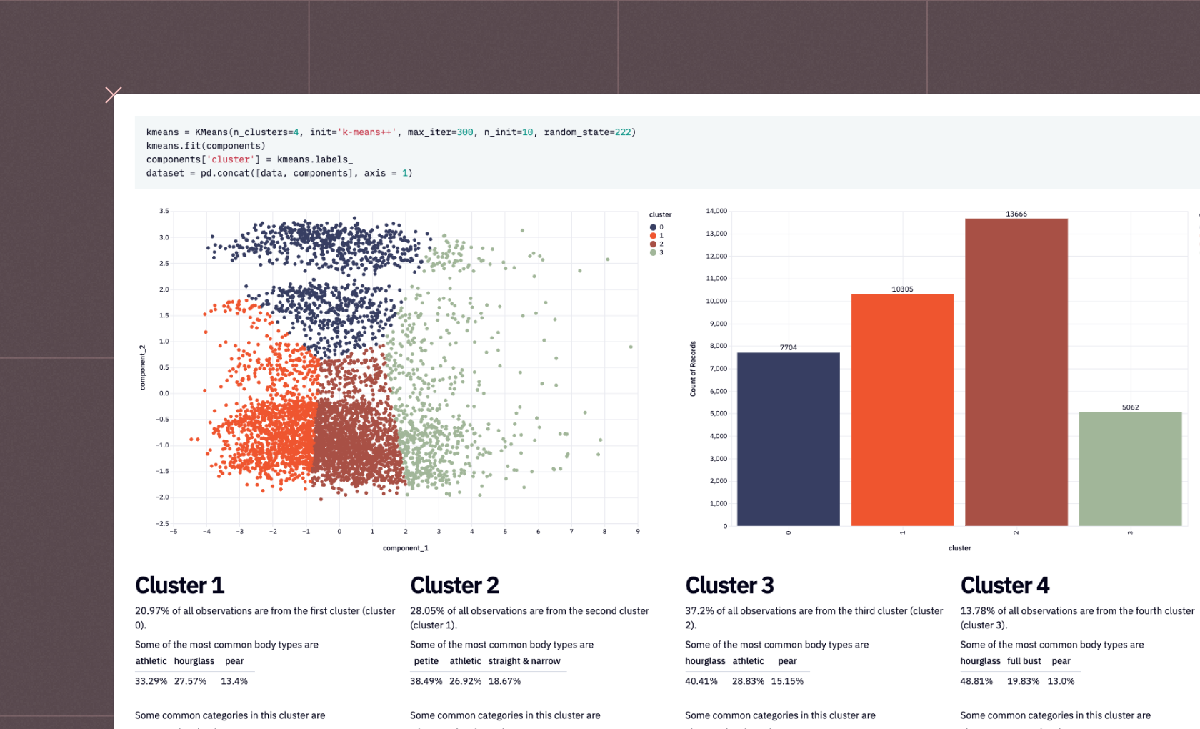
kmeans = KMeans(n_clusters=5, init='k-means++', max_iter=300, n_init=10, random_state=222) kmeans.fit(components) components['cluster'] = kmeans.labels_ dataset = pd.concat([data, components], axis = 1)
This performs the actual K-means clustering on our dataset. It initializes a KMeans object with specified parameters, fits the model to the input data, assigns the resulting cluster labels to each data point, and concatenates the original data with the cluster assignments and component values obtained from dimensionality reduction.
After executing this code, the dataset dataframe will contain the original data columns along with the cluster assignments and the component values. Each data point will have a corresponding cluster label, indicating which cluster it belongs to based on the K-means clustering algorithm.
This code is commonly used in the context of customer segmentation or grouping similar data points together based on their features. By assigning cluster labels to each data point, it becomes easier to analyze and understand the underlying structure and patterns in the data. The resulting dataset can be further analyzed, visualized, or used for downstream tasks such as targeted marketing, personalized recommendations, or customer profiling.
We can in fact visualize this data with Hex’s in-built charting:


Visualizations are helpful, but analysts also like to see the raw numbers and summary statistics. To do that, we’ll build a report for each cluster:
columns_to_report = ['AGE', 'GENDER', 'TOTAL_ORDERS', 'TRAFFIC_SOURCE','MOST_FREQUENT_BRAND','MOST_FREQUENT_CATEGORY']def build_report(cluster):
report = {}
for col in columns_to_report:
group = dataset[dataset['cluster'] == cluster]
info = group.groupby(col)[['USER_ID']].count().sort_values(by = 'USER_ID', ascending = False).reset_index()
info['ratio'] = np.round((info['USER_ID'] / info['USER_ID'].sum()) * 100, 2)
top_5 = info[[col, 'ratio']].iloc[:3].values
report[col] = top_5
report['cluster_ratio'] = np.round((group.shape[0] / dataset.shape[0]) * 100, 2)
return reportreport1 = build_report(0)
report2 = build_report(1)
report3 = build_report(2)
report4 = build_report(3)
report5 = build_report(4)build_report() generates a report for each cluster in a dataset.


The reports can be used to gain insights into the characteristics and patterns of the data points within each cluster, helping in understanding the segmentation of customers or data points based on the chosen columns.
Predicting Customer Segmentation
With our current customers clustered, we can now use that information to try and predict segments for new customers. This will help us to quickly and accurately assign new customers to the most appropriate segment based on their characteristics, behaviors, or preferences. By leveraging the insights gained from clustering our existing customer base, we can streamline the process of understanding and targeting new customers.
features = [{
    "AGE": age,
    "GENDER": gender,
    "COUNTRY": country,
    "TOTAL_ORDERS": total_orders,
    "TRAFFIC_SOURCE": traffic_source,
    "MOST_FREQUENT_BRAND": favorite_brand,
    "MOST_FREQUENT_CATEGORY": favorite_category,
}]
user = pd.DataFrame(features)
encoder = LabelEncoder()# Encode categorical variables
user["GENDER"] = encoder.fit_transform(user["GENDER"])
user["COUNTRY"] = encoder.fit_transform(user["COUNTRY"])
user["TRAFFIC_SOURCE"] = encoder.fit_transform(user["TRAFFIC_SOURCE"])
user["MOST_FREQUENT_BRAND"] = encoder.fit_transform(user["MOST_FREQUENT_BRAND"])
user["MOST_FREQUENT_CATEGORY"] = encoder.fit_transform(user["MOST_FREQUENT_CATEGORY"])The purpose of this code is to prepare our new user profile data for further analysis or prediction. By encoding the categorical variables as numerical values, the data becomes suitable for machine learning algorithms that require numerical inputs.
We can then use it to make predictions:
if make_prediction:
    user_data = {}
    # loop through all the columns present in the original encoded dataframe
    for column in data.columns:
        # if the column is already present in the `user` dictionary (from code cell 40)
        if column in user_dict:
            # then add the data to the user_data dictionary
            user_data[column] = user_dict[column]
        # if the column is not in the dataframe
        else:
            # add the column to the dataframe and set the value to 0 (since it's not present)
            user_data[column] = 0
# create an updated user_data dataframe
user_data = pd.DataFrame([user_data]) # transform features into components
scaled_user_data = scaler.transform(user_data)
user_components = reducer.transform(scaled_user_data)
component_df = pd.DataFrame(user_components, columns = ['component_1', 'component_2'])
# predict cluster
cluster = kmeans.predict(component_df)
component_df['cluster'] = cluster
user_df = pd.concat([user_data, component_df], axis = 1)
# find similar users
df1 = user_df
df2 = dataset similarity = cosine_similarity(user_df[['component_1', 'component_2']], dataset[['component_1', 'component_2']])
dataset['similarity_score'] = similarity[0] * 100
top5 = df2.sort_values(by = 'similarity_score', ascending = False).iloc[:5] #.to_dict(orient = 'records')
else:
user_data = None
cluster = None
user_df = pd.DataFrame()
top5 = pd.DataFrame()This code essentially takes a user's data, transforms it into components using the same scaling and dimensionality reduction techniques applied to the original dataset, predicts the user's cluster, and finds the top 5 most similar users based on cosine similarity of their components.
The core of the code is this part:
The
user_dataDataFrame is transformed into components using the following steps:The
scaler.transform()method is applied touser_datato scale the features.The
reducer.transform()method is applied to the scaled data to reduce the dimensionality and obtain the user's components.The resulting components are stored in a DataFrame called
component_dfwith columns 'component_1' and 'component_2'.
The
kmeans.predict()method is used to predict the cluster to which the user belongs based on their components. The predicted cluster is added as a new column 'cluster' to thecomponent_df.The
user_dataandcomponent_dfDataFrames are concatenated along the column axis to create a new DataFrame calleduser_df, which contains both the user's data and their components.The code then finds similar users to the given user:
The cosine similarity between the user's components and the components of all users in the
datasetis calculated usingcosine_similarity().The similarity scores are added as a new column 'similarity_score' to the
datasetDataFrame.The top 5 most similar users are retrieved using
sort_values()andiloc[]on thedatasetDataFrame, and the result is stored intop5.
The resulting user_df DataFrame contains the user's data along with their components and predicted cluster, while the top5 DataFrame contains the top 5 most similar users to the given user.
Customer segmentation using Python and tools like Hex empowers businesses to unlock the full potential of their customer data. By leveraging advanced clustering techniques like K-Means, businesses can gain deep insights into their customers, make data-driven decisions, and create targeted strategies that drive customer satisfaction and business success.
See what else Hex can do
Discover how other data scientists and analysts use Hex for everything from dashboards to deep dives.
Ready to get started?
You can use Hex in two ways: our centrally-hosted Hex Cloud stack, or a private single-tenant VPC.