Collaborative filtering

Izzy Miller
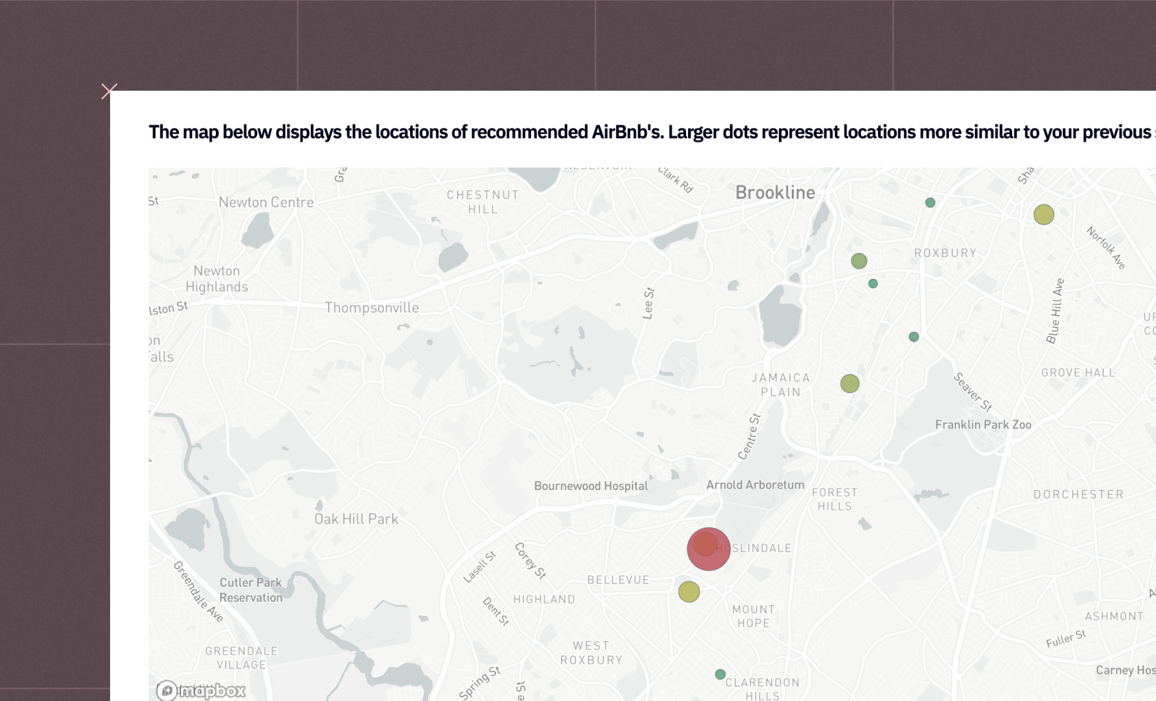
Understand how collective user tastes can be used to find products that are similar to each other and make personalized recommendations based on purchase history. Hex ma...
How to build: Collaborative filtering
Collaborative Filtering (CF) is a technique recommender systems leverage to predict user preferences by identifying similarities between users or items and then using those similarities to suggest items a user may want. It also predicts a user's interests or preferences by gathering behavior patterns of users who share similar interests. One fundamental assumption is that if user A shares preferences with user B on certain items, A has similar preferences to B on other items.
The collaborative filtering technique predicts user preferences by collecting input from multiple users, analyzes similarities between users or items based on their interactions, and recommends items liked by similar users or the user in question. Collaborative filtering predicts what you'll like based on what similar users enjoyed, recognizes the behavior pattern by analyzing past user ratings or purchases to find users with similar tastes, and then recommends items those users liked. For example, find friends with good food taste and ask for their suggestions!
Here, you will learn about various types of collaborative filtering techniques, and algorithms to build a recommendation engine with Python and Hex. You will also see various evaluation metrics to test collaborative filtering.
Types of Collaborative Filtering
There are mainly three types of Collaborative Filtering methods:
User-based Collaborative Filtering
User-based collaborative filtering treats you like a picky eater by understanding what other users with similar tastes enjoyed in the past (their ratings or purchases) and recommends items for you.
Pros:
Serendipity: Discovers unexpected items you might enjoy based on similar users' tastes.
Effective for niche interests: Works well for finding recommendations in specific genres or subcultures with a dedicated user base.
Cons
Cold start problem: New users need more comparative data, making recommendations difficult.
Sparsity: When few users have rated specific items, accurate recommendations become challenging.
Scalability: Finding similar users gets computationally expensive with a massive user base.
Item Based Collaborative Filtering
Item-based collaborative filtering (IBCF) is like asking, "What else goes well with this?" Instead of focusing on similar users, it recommends items users enjoyed alongside what they liked previously or the content they watched the most. IBCF analyzes past user data to find items frequently purchased or rated together with your initial item (e.g., movies often watched after a specific one).
Pros:
Less susceptible to cold start problem: New items can be recommended based on their similarity to existing items.
Handles data sparsity better: Even with limited ratings for specific items, it recommends based on similar, well-rated items.
Efficient for large datasets: Finding similar items is generally faster than finding similar users, especially with a massive user base.
Cons:
Limited to existing item relationships: Can't recommend entirely new categories or items outside the current network of behavior.
Overspecialization: Users might get stuck in an echo chamber of similar items, limiting exposure to diverse recommendations.
Model-based Collaborative Filtering
Model-based collaborative filtering (MBCF) takes a more scientific approach compared to user-based or item-based methods. It utilizes machine learning algorithms to analyze massive user-item interaction data (ratings, purchases, views, etc.). The ML algorithm captures hidden patterns based on user preferences, item characteristics, and their interrelation. It can then be used to predict a user's preference for any item, even if they haven't interacted with it before. MBCF is like having a personalized taste profiler that goes beyond solely similarities and considers multiple factors to make better recommendations.
Pros:
Scalability: Handles large datasets efficiently, making it suitable for platforms with millions of users and items.
Cold start problem mitigation: Can recommend new items even with limited user data, as the model learns from broader patterns.
Flexibility: Can incorporate additional data beyond user-item interactions, like demographics or item features, for richer recommendations.
Cons:
Interpretability: The model predictions are difficult to interpret, making it challenging to explain recommendations or identify potential biases.
Data Dependence: Relies heavily on the quality and quantity of training data.
Overfitting: If the model focuses too much on specific patterns in the training data, it might not identify new or unseen user-item interactions accurately.
In other words, model-based CF offers powerful recommendation capabilities but requires cautious implementation and continuous monitoring to ensure it delivers valuable and unbiased suggestions.
Techniques and Algorithms for Collaborative Filtering
Memory-based CF
Memory-based collaborative filtering (MBCF) is a technique for recommender systems that relies on past user-item interactions to predict user preferences and suggest relevant items. Instead of building complex models, it leverages stored user data to find similarities and make recommendations. Two of the main memory-based approaches are:
User-based CF: Focuses on finding users with similar interests to the target user and recommends items that similar users have enjoyed.
Item-based CF: Focuses on finding items similar to items the target user has interacted with and recommends these similar items to the user.
In MBCF, choosing the right similarity metric is crucial for identifying similar users or items and generating recommendations. Two commonly used metrics are:
Cosine Similarity: Cosine Similarity measures the directional similarity between two vectors representing user or item profiles. This metric relies on the angles between these vectors, not their magnitudes, and considers how items are rated together, not the specific rating values.
Pearson Correlation: Pearson Correlation measures the linear correlation between two user or item rating vectors. This metric calculates the closeness between the ratings of two users or items that vary simultaneously.
Model-based CF (MBCF)
MBCF takes a more sophisticated approach than memory-based methods by leveraging machine learning algorithms to analyze vast amounts of user-item interaction data (ratings, purchases, views) and builds a model to predict user preferences.
Data Analysis: The model is trained on historical data, uncovering hidden patterns and relationships between users, items, and their interactions.
Model Learning: Algorithms like matrix factorization or deep learning techniques identify these patterns and encode them into a mathematical model.
Prediction and Recommendation: Once trained, the model can predict a user's rating or preference for any item, even if they haven't interacted. This feature allows the system to recommend relevant items the user may enjoy.
Matrix Factorization Techniques
Matrix factorization (MF) is a popular technique used within MBCF. It decomposes a user-item rating matrix into two lower-dimensional matrices, capturing latent factors that explain user preferences and item characteristics. Here are two factorization methods:
Singular Value Decomposition (SVD): Decomposes the matrix into three matrices: user factors, singular values, and item factors. These factors represent underlying (genres, actors) user rating influencing features.
Alternating Least Squares (ALS): Optimizes the user and item factors iteratively to minimize the prediction error between the actual ratings and the model's predicted ratings.
Deep Learning Approaches
Deep learning models, like autoencoders or neural networks, can be powerful tools for MBCF. They can learn complex relationships between users, items, and additional data sources (text descriptions, images) to make more personalized recommendations.
Hybrid-Models Combining Collaborative Filtering and Content-Based Filtering (CBF)
Combining CF with CBF can create even more robust recommender systems. CF leverages user-item interactions to identify similar users or items. CBF analyzes item content (descriptions, features) to recommend items similar to those a user liked previously.
Benefits of hybrid models include:
Improved recommendation accuracy: Combines the strengths of both CF and CBF, leading to more relevant suggestions.
Cold start problem mitigation: CBF can recommend new items with limited user data based on content analysis.
Serendipity: Explores connections between user preferences and item characteristics for unexpected recommendations.
By understanding these different approaches, you can leverage the most suitable technique (or a combination) for building effective recommender systems that personalize user experiences and drive engagement.
Evaluation Metrics
Choosing the right metrics is crucial for evaluating the performance of a collaborative filtering (CF) system. The following are some commonly used metrics:
Mean Squared Error (MSE) and Root Mean Squared Error (RMSE)
These metrics calculate the difference between predicted ratings by the CF system and the actual user ratings.
MSE: Calculates the average squared difference between predicted and actual ratings.
RMSE: RMSE is the square root of MSE, easy to interpret as it has the same scale as the ratings.
NOTE: You should minimize MSE and RMSE for better performance while building a recommendation system.
Precision, Recall, and F1-score
These metrics are typically used for binary classification tasks (item recommendation can be seen as classifying items as relevant or not). However, they can be adapted for CF evaluation in some scenarios.
Precision: Measures the proportion of recommended items users liked (relevant).
Recall: Measures the proportion of all relevant items (items the user would like) that the system recommended.
F1-score: Harmonic mean of precision and recall, providing a balanced view of both metrics.
Coverage and Diversity Metrics
These metrics go beyond accuracy and assess the breadth and variety of recommendations. Coverage measures the proportion of items the CF system can recommend. Diversity measures how different the recommended items are from each other. By understanding these metrics and their trade-offs, you can effectively evaluate and improve the performance of your CF system.
Collaborative Filtering with Python and Hex
In this section, you will see a practical implementation of collaborative filtering with the help of Python and Hex. Hex is a modern development environment that provides a similar interface to Jupyter Notebook but it is a lot more capable of developing and deploying interactive Python applications and dashboards. It is a polyglot platform that allows you to write code in different languages within the same development environment. It can connect to various data sources including different databases, data warehouses, and cloud storage. It also provides the no-code visualization capability with the help of its no-code cells. Overall, Hex makes it easy to build a recommendation engine using collaborative filtering with Python, and then deploy it as an interactive web app.
We will try to understand how collective user tastes can be used to find products that are similar to each other and make personalized recommendations based on purchase history. For this, we will use a book purchase dataset. We will be using Python 3.11 and SQL languages throughout this section to create a recommendation app using collaborative filtering.
Let's start with the implementation.
Install and Load Dependencies
To begin with, you need to install a set of Python dependencies that will help you manipulate data and perform collaborative filtering. Although Hex already comes with a lot of Python dependencies preinstalled, you can use the Python Package Manager (PIP) to install the dependencies if they are missing.
$ pip install pandas
$ pip install numpy
$ pip install scikit-learn
Once the dependencies are installed, you can load them into the Hex environment as follows:
import pandas as pd
import numpy as np
import sklearn
from sklearn.decomposition import TruncatedSVD
from collections import Counter
The pandas and numpy libraries will help us to load and preprocess the data while sklearn will help us to create the collaborative filtering model and evaluate that.
Load and Preprocess Data
The aim of our project is to provide users with book recommendations based on their purchase history. To achieve this, we have two tables at our disposal. The first table displays the books each user has read and their corresponding ratings. It can be loaded with the help of a simple SQL SELECT statement as follows:
select * from "DEMO_DATA"."DEMOS"."BOOK_RATINGS"


Meanwhile, the second table offers more detailed information on each book and it can be loaded with the help of the following SQL command:
select * from "DEMO_DATA"."DEMOS"."BOOK_DATA"


Although there could be multiple preprocessing stages involved at this phase depending on the data that you use. But for this data, we mainly need to remove the null values (missing data) that can cause issues in building the recommender system. In our data, columns like USER_ID, Book_title, Title, and RATING contain some null values, we will remove the entire row from the data if any of these columns have a null value. To do so, we can use the dropna() method from pandas as follows:
data.dropna(subset = ['USER_ID', 'Book_title', 'RATING'], axis = 0, inplace = True)
books.dropna(subset = ['Title', 'DESCRIPTION'], axis = 0, inplace = True)
You might see two other arguments that we have used in the dropna() method. The first one is the axis that defines the orientation based on which you would want to remove the null values. If it is set to 0 the entire row containing a null value would be dropped, on the other hand, if it is set to 1 the entire column containing a single null value would be dropped. The inplace argument allows us to make changes in a dataframe and overrides that dataframe with the latest changes.
Note: Usually it is not a good practice to drop the null values if you have a very small number of rows in your data. In that case, you can compute the null values manually or fill them with measures of central tendency. For our data, we have plenty of rows which is why we are dropping the rows containing null values.
Now, to check if there exists any null value in your dataset, you can use the following code:
data.isnull().sum()


By looking at the above image, you may be wondering, "Why haven't we removed the almost 7000 null price values?" Although there are almost 7000 null price values in our dataset, we have decided to keep them since the price variable isn't very important for our project's objective. This allows us to preserve those 6.8k rows in our dataset.
You can also have a look at the number of unique users and products in the dataset using the nunique() method from pandas.
product_count = data['ITEM_ID'].nunique()
user_count = data['USER_ID'].nunique()


Understanding User Taste
To determine the readers who prefer specific books, it is necessary to generate a user-item matrix. This matrix comprises rows that represent books and columns that represent readers, with the values indicating the ratings that each user has assigned to each book. However, since not every user has read all the books, the resulting matrix contains a lot of zeros. A matrix with a significant number of zeros is referred to as a sparse matrix.
To do so, we will create a pivot table that will be the perfect match for creating the sparse matrix. You can create a pivot table in the Hex environment with just a few clicks without any code. Just click on add a new pivot table under the "transform" options in the add cell menu and provide the necessary details to get yourself a pivot table.


Due to the pivot results being returned as a multi-indexed dataframe, we're going to want to flatten it to a single index. In this case, If you look at the columns of the pivot table you'll see USER_ID and RATING_SUM as indexes. You can do so with the help of the following lines of code:
pivot_data = pivot_result.pivoted
pivot_data.columns = pivot_data.columns.to_flat_index()
In the above code, we have simply created a flat index using the to_flat_index() method in pandas.
Memory Based vs Model Based Recommendations
Now that you have the preprocess data, you have a choice to make for collaborative filtering. As you have seen in the previous section there are various methods to perform collaborative filtering. In this case, we're using a model-based approach utilizing TruncatedSVD to compress our sparse matrix into a dense matrix. The model compresses all of the users into 12 latent features per book where this new matrix represents generalized user tastes. By looking at a specific user's purchase history, we can recommend books that are highly correlated with books that the user has already read.
To do so, you simply need to create an object of the TruncatedSVD() model and use the fit_transform() method to create a dense matrix as follows:
svd = TruncatedSVD(n_components=12, random_state=111)
user_taste = svd.fit_transform(pivot_data)
user_taste = pd.DataFrame(user_taste)
user_taste.index = pivot_data.index


Making Recommendations
Now it is time to make some recommendations for the customers. Let's start with creating a correlation matrix of related books. A correlation tells us how strongly two or more things relate to each other and in this case, highly correlated books mean they are similar in content.
corr_mat = np.corrcoef(user_taste)
matrix = pd.DataFrame(corr_mat, columns = list(user_taste.index), index = user_taste.index)
matrix.shape


In the above code, we have first used the corrcoef() method to calculate the correlation matrix, and then we have created a pandas dataframe from that matrix. The actual matrix looks like this:


Now we will use different components from hex such as buttons and sliders to make our work easy. We will use the following controls:
Adjust the
number of recommendationsslider to determine the number of recommended books.Use the
Gram countslider to set the level of detail in each topic for the recommended books.Click the button to select a random user and generate book recommendations for them.
The selection slider for number of recommendations looks something like this:


As soon as you select the appropriate value, you can use the following lines of code to generate the recommendations for a specific user.
def random_purchases:
	users_with_more_than_one_purchase = list(set(data.set_index('USER_ID')[(data['USER_ID'].value_counts() > 1)].index))
	random_user = np.random.choice(users_with_more_than_one_purchase)
	user_data = data[data['USER_ID'] == random_user]
	username = user_data['NAME'].to_list()[0]
	items = list(set(user_data['ITEM_ID'].to_numpy()))
	book_name = list(set(user_data['Book_title'].to_numpy()))
	purchased_products = np.random.choice(items, size = 5)
	print(f"User {username} has purchased {len(items)} books {book_name}")
	most_similar = {}
	all_recommendations = []
	for product in purchased_products:
    	# filter the dataframe by product and sort by the similarity score
    	filtered = matrix[product].sort_values(ascending = False)
    	filtered.drop(product, axis = 'index', inplace=True) # drop any repeat purchases
    	# return the top 10 most similar products
    	top10 = list(filtered.index[1:11])
    	# along with their similarity score
    	scores = filtered.iloc[1:11].to_list()
    	# add the top10 products and their similarity scores to the dictionary
    	most_similar[product] = list(zip(top10, scores))
    	all_recommendations.extend(top10)
recommendations = Counter(all_recommendations)
recommended_books = recommendations.most_common()[:num_of_recs]
recommended_books = [val[0] for val in recommended_books ]
else:
recommended_books = []
book_name = []
items = []
user_data = pd.DataFrame()
username = None
purchased_products = []


In the above code, if the random_purchases is set to 0 then there would be no predictions for the user as specified in the else block of the code. Otherwise, the code would run and it would filter out the top 10 recommendations for a selected customer.
Then we can filter out the additional data from the original dataframe with the help of the following lines of code:
recommended_products = data[data['ITEM_ID'].isin(recommended_books)] if recommended_books is not None else pd.DataFrame()

Next, we will filter the author, description, and category. To do so, define the following lines of code to preprocess the text and load the necessary text processing dependency:
import re
from sklearn.feature_extraction.text import TfidfVectorizer
clean = lambda text: re.sub("[^0-9A-Za-z ]", "", text)
Next, we will define a few methods that will filter down the required details by simply filtering the dataframes.
def get_author(book):
	author = clean(str(list(books[books["Title"] == book]["AUTHORS"])))
	if len(author) == 0:
    	return None
	else: return author
def get_description(book):
desc = list(books[books["Title"] == book]["DESCRIPTION"])
if len(desc) == 0:
return 'No description'
else: return desc[0]def get_category(book):
cats = clean(str(list(books[books["Title"] == book]["CATEGORIES"])))
if len(cats) == 0:
return None
else: return cats
def get_book_info(book_names):
	authors = [ get_author(title) for title in book_names ]
	description = [ get_description(title) for title in book_names ]
	categories = [ get_category(title) for title in book_names ]
	return authors, description, categories
We will now call the get_book_info() method to get the author, description, and category.
original_authors, original_description, original_categories = get_book_info(book_name)
original_info = list(zip(book_name, original_authors, original_description, original_categories))
has_book_info = lambda book: not books[books["Title"].isin(book_name)].empty
Now, we will define the favorite_category based on the most common items for the selected user.
favorite_category = Counter(original_categories).most_common()
favorite_category = [category for category in favorite_category if category[0] is not None][0][0] if len(favorite_category) > 0 else 'No categories'
Finally, we will get the final recommended book, author, and description with the help of the following lines of code:
rec_book_names = list(recommended_products["Book_title"].unique()) if not recommended_products.empty else [None]
rec_book_authors, rec_book_description, rec_book_categories = get_book_info(rec_book_names)
rec_info = list(zip(rec_book_names, rec_book_authors, rec_book_description, rec_book_categories))
Next, we will define a Python method get_tfidf_top_features() that uses the TfidfVectorizer to convert text into vectors and then finds the most important vectors among all, and then returns them. This will help us understand what the most common themes and topics are in the recommended books.


import numpy as np
from sklearn.feature_extraction.text import TfidfVectorizer
def get_tfidf_top_features(documents, n_top=8):
	tfidf_vectorizer = TfidfVectorizer(
    	stop_words="english", ngram_range=(gram, gram)
	)
	tfidf = tfidf_vectorizer.fit_transform(documents)
	importance = np.argsort(np.asarray(tfidf.sum(axis=0)).ravel())[::-1]
	tfidf_feature_names = np.array(tfidf_vectorizer.get_feature_names_out())
	return tfidf_feature_names[importance[:n_top]]# Answer
Finally, to get the highly recommended topics, we will pass the description obtained from the previous stage to this get_tfidf_top_features() method and it will give us the highest recommended topics.
This is it, you have now created a product recommender based on collaborative filtering. But there is obviously more that you can achieve with Hex. When you head over to the App Builder section in the Hex environment, you will see that a dashboard might have already been created for you. You can adjust the components of this dashboard by dragging and dropping them to the desired location. Once you feel that the dashboard looks good enough, you can click on the publish button to publish the app in Hex.


This is it, this is how easy it is to create the recommender system and deploy it in a few simple clicks.
By leveraging Hex's interactive components and no-code capabilities, the recommender system can be easily customized and deployed as a user-friendly web app. With the right combination of techniques, evaluation metrics, and best practices, collaborative filtering empowers businesses to deliver highly relevant recommendations, enhance user engagement, and drive business growth.
See what else Hex can do
Discover how other data scientists and analysts use Hex for everything from dashboards to deep dives.


Ready to get started?
You can use Hex in two ways: our centrally-hosted Hex Cloud stack, or a private single-tenant VPC.