Customer lifetime value Dashboard

Any business has a mix of customers. Some customers buy products regularly, some make purchases less frequently, and some new customers are trying the products for the first time. According to the 80/20 rule from Italian economist Vilfredo Pareto, 80 % of the profit of any business comes from the 20% of the customers (that are regular).

As a business, you want to know who these 20% of valuable customers are.

Customer lifetime values analysis (CLV) helps businesses understand how much a customer is worth to them. CLV is an analytical approach that helps businesses estimate the total monetary value a customer can bring to the business over the entire relationship duration. It is one of the most important concepts in business strategy as it helps businesses understand the long-term value of acquiring and retaining customers. Once businesses identify what customers are very important to them, they can make strategic decisions regarding marketing, customer acquisition, and customer retention.

This article will teach you more about this technique and how to build a CLV analysis dashboard using Python and Hex.

Customer Lifetime Value Analysis

CLV is an effective way to calculate churn risks and predict customer behaviors. Two different types of churn are normally seen in any business.

First is contractual churn, where customers have subscriptions to a certain product or service for a specific period of time, and as the subscription end nears the churn risk appears to be more transparent. Second is non-contractual churn where instead of focusing on the subscription end, we analyze the customers purchasing behavior and make distributional assumptions. While the earlier one is easy to model and make predictions, the latter is more complex. CLV can be performed in both contractual and non-contractual settings.

CLV holds a lot of importance for a business due to the following reasons:

• Strategic Resource Allocation: CLV helps identify the customers with the best monetary value to the business. This can help businesses to allocate resources more effectively by focusing on high-value customers. Businesses need to prioritize their marketing efforts and resources only on the customers likely to generate the most revenue over the long term.

• Marketing Optimization: Based on the results from CLV, businesses can tailor their marketing strategies, such as optimizing advertising spend, developing targeted campaigns, and creating personalized offers to attract and retain valuable customers.

• Customer Segmentation: CLV businesses can easily identify customers with similar behavior and create segments for them. This helps them to create different strategies for each group to improve customer satisfaction and retention.

• Optimizing Customer Acquisition Cost (CAC): By comparing the results of CLV with the customer acquisition cost (CAC) businesses can assess if acquiring new customers is cost-effective or maintaining the existing ones.

• Forecasting Revenue and Growth: CLV helps clear the business perspective; with this forward-looking perspective, businesses can forecast future revenue and growth. This offers insights for long-term planning and strategic decision-making and aids in developing reasonable and attainable corporate goals.

These are just a few important points regarding CLV; there are, of course, many other valuable things that CLV brings to a business.

Different Methods of CLV

Now that you know what CLV is and why it is important for businesses, this is time to look into some of the most popular methods used for CLV analysis. One important thing to note about CLV is that to calculate it, you need historical data about the customers, which is impossible for new customers. Due to this reason, it is preferable to use traditional algorithms like the BG/NBD model. While machine learning models are used for the data with new customers.

• Buy Till You Die: BTYD is a framework designed for estimating and predicting the CLV, especially for non-contractual customers. This model analyzes customer purchasing behavior over time and assumes that customers will continue to purchase until they die or become inactive. This model employs the probability distribution such as the Poisson distribution for the transaction counts and the Exponential distribution for inter-purchase times, to model the likelihood of customers making repeat purchases. By using predictive analytics, these models try to forecast future customer behavior and estimate the expected number of future purchases from each customer.

• BG/NBD Model: The Beta Geometric/Negative Binomial Distribution (BG/NBD) is a widely used model in customer analytics for churn analysis and CLV. This model combines the elements of the Beta distribution and the Negative Binomial distribution to characterize customer behavior. It focuses on Predicting the probability of the customers being dead or inactive and the distribution of the number of transactions made by active customers.

• Gamma-Gamma Model: The Gamma-Gamma model is based on Gamma distribution and is designed to estimate customers' monetary or average transaction value in non-contractual settings. This model is often deployed with the BG/NBD model to increase the efficiency of CLV analysis. This model considers two different things: the number of transactions that a customer makes and the amount of money spent in each transaction. The Gamma-Gamma model is very useful for businesses where consumers have a range of buying habits.

• Predictive Modeling: In the case of non-contractual and non-subscription settings, the predictive models are specially used for the data that also contains some new customers. As part of this technique, different ML algorithms like clustering, classification, and regression are used depending on the use case.

Some Common Metrics For CLV

Some of the most common CLV metrics used by the above-mentioned algorithms are as follows:

1. Frequency: It is the count that the customers make after the initial purchase of the product.

2. Recency: It is the duration in days between a client’s initial and most recent transactions.

3. Longevity (denoted by T): It is the number of time periods since the customer’s first purchase and the last observed date in the analysis.

4. Monetary Value: It is the average amount that a customer spends on a transaction.

Implementing CLV with Python and Hex

Now that you know different methods to perform the CLV, it is time to implement these methods on some real-world data. In this section, we will prepare a dashboard using the Hex platform. Hex is an interactive development platform that allows you to write and run the code in an interactive environment. It allows you to easily run and debug your code with the support of no-code visualization. Hex can also support connections to different data storage mechanisms, such as databases and cloud storage to easily import and export data to various platforms.

We will use the Python 3.11 language and Hex as a development platform for development. We will use the Python Package Manager (PIP) to install the Python dependencies. The data we will use is from an online retail store and stored in the Snowflake warehouse.

Install and Load Dependencies

To begin with, let’s install all the necessary Python dependencies with the help of PIP as follows:

$ pip install pandas numpy
$ pip install Lifetimes

The Pandas as Numpy libraries will be used for manipulating data and Lifetimes library will be used to perform different CLV algorithms as it has the implementation of them all.

Once installed, you can import the dependencies in the Hex environment as follows:

import lifetimes

import pandas as pd
import numpy as np

from lifetimes import BetaGeoFitter
from lifetimes import GammaGammaFitter

Load and Explore the Data

Our data is stored in a Snowflake warehouse, we can easily read it into the Hex environment with the help of a simple SQL statement. The data is always loaded into a Pandas DataFrame which makes the data processing and manipulation a lot easier.

select * from "DEMO_DATA"."DEMOS"."ONLINE_RETAIL"

Next, we will use some inbuilt Python methods to understand the data. Let’s begin with checking the descriptive statistics of all the numerical features in the dataset using the describe() method from Pandas.

df.describe()

As you can see in the above image, the Quantity and UnitPrice columns have a really small value for mean while their min and max values are quite extreme. This shows the presence of outliers in the dataset.

Next, we will check the presence of NaN (Null) values in the dataset. To do so you can use the install () method to get all the null values in a column and the sum() method to get an aggregate sum for the same.

df.isnull().sum()

The CustomerID and Description columns contain some NaN values that we will have to remove to proceed with CLV analysis.

Data Cleaning

As part of data cleaning, we will address the outliers and the null values in the dataset. We will perform the following operations to clean the dataset:

• Keep the data rows where at least one order is placed less than 0 does not make any sense.

• Remove the items whose cost is less than 0 i.e. they do not cost anything.

• Remove all the returned orders.

• Drop all the null values in the dataset as we have plenty of data.

• Convert CustomerID from Float to string.

• Remove the time component from the InvoiceDate feature.

All these changes can be made using dataframe filtering and basic Pandas functions as follows:

df = df[df['Quantity'] > 0 ] # takes care of unaccounted returns or cancellations
df = df[df['UnitPrice'] > 0] # remove items that appear not to cost anything
df = df[~df['InvoiceNo'].str.contains("C",na=False)] # drop returned items
df.dropna(inplace=True) # drop all nulls
df['CustomerID'] = df['CustomerID'].astype(str) # convert customerID to a string
df["InvoiceDate"] = pd.to_datetime(df["InvoiceDate"]).dt.date # removes time component from date

Next, we will create a Python function for detecting the outliers using the Interquartile range. All the values that fall below Q1 and above Q3 are considered outliers. So we will create a method to calculate the lower (Q1) and upper (Q3) limit of our data.

def outliers(values):
	# Calculate the 5th and 95th percentiles of the input values
	q1, q3 = np.percentile(values, [5, 95])

	# Calculate the interquartile range (IQR)
	iqr = q3 - q1

	# Calculate the lower and upper outlier limit
	lower = q1 - (1.5 * iqr)
	upper = q3 + (1.5 * iqr)
	return lower, upper

Finally, we will create another Python method that will take a dataframe feature, will calculate the lower and upper limit for that feature and then it will filter the values that fall past these limits.

def remove_outliers(frame, column):
	# Calculate the lower and upper outlier limit for the specified column
	lower, upper = outliers(frame[column])

	# Create filters that remove all rows that fall outside of these limits
	lower_mask = frame[column] > lower
	upper_mask = frame[column] < upper

	# Apply the filters to the dataset
	cleaned_frame = frame[lower_mask & upper_mask]
	return cleaned_frame

Since outliers are present in the Quantity and UnitPrice columns, we will apply the above method to these columns.

data = remove_outliers(df, 'Quantity')
data = remove_outliers(data, 'UnitPrice')

Once the outliers are removed, we can again check the descriptive statistics of the data.

data.describe()

You can notice in the above image that the outliers are removed as there are no extreme values present in any of these features.

Next, we will create an extra column TotalPrice that will be the result of the multiplication of UnitPrice and Quantity.

data['TotalPrice'] = data['UnitPrice'] * data['Quantity']

Now, before applying any CLV analysis method, we will check the total number of unique customers and the total revenue earned from all orders made.

customers = data['CustomerID'].nunique()
revenue = data['TotalPrice'].sum()

Buy Till You Die Model

Now that you have a clean dataset and know a bit about what information it contains, it is time to start our analysis. To be specific, we will be using the BG/NBD and Gamma-Gamma model for the the same. For applying this analysis, we will be selecting one customer from the dataset. Once the customer is selected, we will get all the metrics (mentioned in the previous section) for that customer.

if cust:
	# Select a random customer from the dataset
	customer = np.random.choice(data["CustomerID"])
else: customer = '13124.0'

# Filter the dataset to only include data for the selected customer
customer_data = data[data["CustomerID"] == customer]

# Find the date of the customer's first purchase
birth = customer_data["InvoiceDate"].min()

# Find the date of the customer's most recent purchase
latest = customer_data["InvoiceDate"].max()

# Find the date of the most recent purchase in the entire dataset
last_global_purchase = data["InvoiceDate"].max()

# Calculate the customer's CLV (Customer Lifetime Value) summary data
customer_clv = lifetimes.utils.summary_data_from_transaction_data(
	customer_data,
	"CustomerID",
	"InvoiceDate",
	"TotalPrice",
	observation_period_end=last_global_purchase,
)

# Extract the recency value from the CLV summary data
recency = customer_clv["recency"][0]

# Extract the frequency value from the CLV summary data
frequency = customer_clv["frequency"][0]

# Extract the longevity value (time since first purchase) from the CLV summary data
longevity = customer_clv["T"][0]

# Extract the monetary value from the CLV summary data
monetary_value = customer_clv["monetary_value"][0]

As you can see in the above code chunk, we are first extracting the birth date, date of the customer’s first purchase, date of the customer’s most recent purchase, and the date of the most recent purchase in the entire dataset. Then we pass the required details such as CustomerID, InvoiceDate, TotalPrice, and last_global_purchase, to the summary_data_from_transaction_data() method from lifetime.utils to get the CLV summary for the selected customer.

To apply this for all the customers, we need to call the summary_data_from_transaction_data() method over the entire dataset.

clv = lifetimes.utils.summary_data_from_transaction_data(data,'CustomerID','InvoiceDate','TotalPrice',observation_period_end='2011-12-09')
clv = clv[clv['frequency']>1] # We want only customers who've shopped more than 2 times

This is it, you now have a new dataframe (clv) that will be used further for analysis.

BG/NBD Model for Predicting the Number of Purchase

Now, we will use the BetaGeoFitter to apply the BG/NBD model on the newly created dataframe. This model will try to predict the number of purchases for each customer for a defined period.

bgf = BetaGeoFitter(penalizer_coef=0.001)
bgf.fit(clv['frequency'], clv['recency'], clv['T'])

Once you have trained the model, you can choose the number of months to look into the future. This is where you can use the feature from Hex to define a slider to select the number of months (eg. 8).

After selecting the number of months, you can use the conditional_expected_number_of_purchases_up_to_time() method to predict the number of purchases for the defined months.

t = months * 30 # 30 day period
clv['expected_number_of_purchases'] = bgf.conditional_expected_number_of_purchases_up_to_time(t, clv['frequency'], clv['recency'], clv['T'])
clv.sort_values(by='expected_number_of_purchases',ascending=False).head(5)

Gamma - Gamma Model

Finally, we will implement the Gamma-Gamma model to estimate how much a customer is likely to spend on average in future purchases. This model gives the estimation of average customer spend, this can really help businesses to tailor their marketing efforts and promotions accordingly.

The Gamma-Gamma model assumes that there is no correlation between the monetary value and the purchase frequency. This essentially means that the amount spent on purchase does not directly depend on the number of times the customer visits the store. To check the correlation between these two features, you can use the Corr() method.

clv[['frequency','monetary_value']].corr()

Since no correlation can be seen between these two columns, we are good to go with the Gamma-Gamma model. To apply this model, you can use the following code:

gf = GammaGammaFitter(penalizer_coef=0.01)
ggf.fit(clv["frequency"],
    	clv["monetary_value"])

Customer Lifetime Value for Selected Months

We will use these trained models (Gamma-Gamma and BG/NBD) to calculate the CLV for each customer. We can calculate the CLV for the selected number of months as follows:

lifetime_value = clv.copy()
lifetime_value["Lifetime_value"] = ggf.customer_lifetime_value(
	bgf,
	lifetime_value["frequency"],
	lifetime_value["recency"],
	lifetime_value["T"],
	lifetime_value["monetary_value"],
	time = months,
	freq="D",
	discount_rate=0.01,
)

Finally, to check the calculated values, you can use the following line of code:

lifetime_value[['monetary_value', 'expected_number_of_purchases', 'Lifetime_value']].sort_values('Lifetime_value',ascending=False).head()

Customer Segmentation for Selected Months

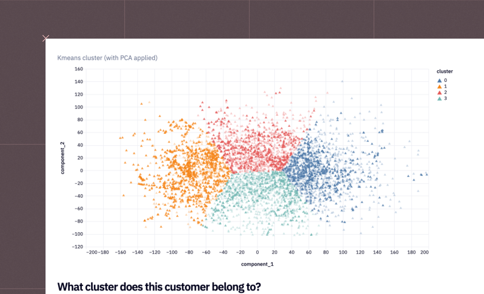
You can also segregate the customers into four different groups i.e. “Hibernating”, “Need Attention”, “Loyal Customers”, and “Champions” (arranged from least valuable to the most) based on their N-month (eg. 6-month) Customer Lifetime Value (CLV).

# The following code snippet assigns customer segments based on their 6-month Customer Lifetime Value (CLV) # by dividing the customers into 4 equal groups (quartiles) and labeling them accordingly. lifetime_value["Segment"] = pd.qcut( lifetime_value["Lifetime_value"], # The CLV data to be divided into quartiles 4, # The number of equal groups (quartiles) to divide the data into labels=[ "Hibernating", # Label for the lowest quartile (25% of customers with the lowest CLV) "Need Attention", # Label for the second quartile (25% of customers with the next lowest CLV) "Loyal Customers", # Label for the third quartile (25% of customers with the next highest CLV) "Champions", # Label for the highest quartile (25% of customers with the highest CLV) ], )

To check the segments for the customers, you can use the following line of code:

lifetime_value[['expected_number_of_purchases', 'Lifetime_value', 'Segment']].sort_values('Lifetime_value',ascending=False).head()

Group by Segment for the Next Selected Months

You can also calculate an aggregate across all the categories in the data to get an overall picture. You can do so with the help of the following SQL command:

SELECT
	Segment,
	AVG("T") AS "T",
	AVG(recency) AS recency,
	AVG(frequency) AS frequency,
	AVG("Lifetime_value") as "Lifetime_value", AVG(monetary_value) as monetary_value, AVG(expected_number_of_purchases) as expected_number_of_purchases
FROM lifetime_value
GROUP BY Segment

Finally, to check the average lifetime value across different customer segments, you can use the following code:

segment_stats['Lifetime_value'] = segment_stats[['Lifetime_value']].apply(lambda x: round(x, 2))

As you can see in the above graph, the dataset conatains more number of champions as compared to other categories.

This is it, you have now created your dashboard for Customer Lifetime Value Analysis using Python and Hex. You have seen a step-by-step guide to preparing a CLV dashboard using Python and Hex. This information will allow you to track the number of purchases a customer will make in a specific timeframe.

By looking into the metrics of recency, frequency, monetary value, and customer age, you can gain a deeper understanding of customer’s purchasing behavior and can identify segments of different types of customers. This will help you to identify the right marketing strategy such as launching targeted campaigns if a customer fails to purchase before the designated window closes, etc. leading to more value to the business.