Time Series Forecasting with Prophet

Everyone wants to see the future. And that’s exactly what you can do with time series forecasting.

Time series forecasting problems are more complex predictive modeling problems than classification problems or straight regressions, as they add the complexity of sequence dependence among the input variables. They also have the nuance that the results obtained from the time series forecasting are variable given the nature of time.

Still, time series forecasting can be helpful in a number of use cases, such as predicting stock market trends, forecasting weather patterns, anticipating consumer demand in retail, managing inventory in supply chain operations, predicting energy usage, forecasting sales revenues, anticipating traffic flow patterns, predicting currency exchange rates, planning agricultural yields, and estimating future healthcare trends, where these predictions can provide a reasonable approximation of the future truth.

While machine learning algorithms like linear regression, random forest, and neural networks are preferred for data that has multiple explanatory variables and you want to model their relationship with the target variable, traditional models like Prophet, ARIMA, SARIMAX, or Vector Autoregression are used to make predictions entirely based on the time-dependent features such as trends and seasonality.

In this article, you will learn about time series forecasting and use the Prophet model to forecast the future values of a time-dependent dataset with the help of Python and Hex.

Understanding Time Series Data

Time series data has some properties that make it different from the other data types. You must understand these properties to use the best algorithm for modeling. Some of the most important characteristics of time series data are:

• Temporal Ordering: The data in time series is always ordered chronologically, i.e., the observations in the data are always recorded at fixed or uneven time intervals. This order is necessary as it represents the evolution of the phenomenon being measured. For example, measuring a temperature each day represents the progression over time, and it is considered a time series problem.

• Trend: Trend represents the long-term change in the value of time series data over time. A trend can have three possible values: an increasing value represents the uptrend, a decreasing value represents the downtrend, and a constant value represents the trend remaining constant. Also, a trend can be linear, exponential, or follow more complex patterns.

• Seasonality: Seasonality refers to the property of time series where the data show the repeating patterns over a fixed period. These patterns can occur daily, weekly, monthly, or regularly. The reason for these periodic patterns can be holidays, seasonal factors, natural phenomena, and other external factors. One such example of seasonality is sales of AC explode every summer.

• Cyclic Patterns: Cyclic patterns are long-term fluctuations in data with no set repetition and seasonality. These patterns are not as regular as seasonal effects, but they usually last for longer periods. One type of cyclic pattern is the economic cycle.

• Residual: Once the trend and seasonality components are extracted from the time series data, only noise and irregularities remain that are random fluctuations or disturbances these irregularities are what we call residuals. These irregularities are highly unpredictable and can be caused by various factors, such as measurement errors or random events.

• Missing Values: Sometimes, there could be data collection errors or gaps in recording while collecting the data for time series analysis these issues lead to missing values in the data. Handling missing values appropriately is crucial for maintaining the integrity of the time series.

• Stationarity: When stationarity is present in the time series data, it does not change over time. A stationary time series has a constant mean and variance, which makes it easier to model and analyze. Most of the time, the series assumes the presence of stationarity as it helps them to model the data easily.

Now, you might be wondering why there are a lot of components in time series and how you can identify each of them in your data. To address this, you must understand that the main components that help in modeling are Trend, Seasonality, and Residual. To check this in your data, use the Seasonal-Trend Decomposition using Loess (STL) decomposition. It helps you to easily identify the Seasons, Trends, and Residuals in the patterns in your data. Likewise, the Augmented Dickey-Fuller (ADF) test and the Kwiatkowski-Phillips-Schmidt-Shin (KPSS) test are used to identify the stationarity components in the data.

Introduction to Prophet

Time series forecasting can be conducted with the help of several models depending on your data type. Each method has its own hyperparameters whose optimal value you need to identify for better forecasting. However, continuous research in the field has produced many new models that can make your entire time series forecasting a lot easier. One such model is Prophet developed by Facebook. It is an open-source model that is used for making a forecast for univariate time series data. For data that has a trend and seasonal structure, it can automatically find a good set of hyperparameters for the model for efficient forecasting. It is completely automatic you just need to train the model with simple steps and use it to make forecasts on new data.

Prophet can be used with languages like Python and R. It provides the same model APIs as sklearn, i.e., you just need to create an object of Prophet and then call the fit() and predict() methods to train the model and make the forecast, respectively.

Creating a Time Series Forecasting Model with Prophet and Hex

Now that you know a bit about time series forecasting and the different components of time series, it is time to check out the practical implementation of time series forecasting. We will use the Prophet model to forecast the daily temperature across various cities.

This section will use Python 3.11 language and Hex as a development platform. Hex is an interactive development environment that allows you to read and write data directly from data warehouses, databases, and cloud storage. It can easily be integrated with different Python libraries, such as Prophet, for making the forecast. It is also a polyglot platform that allows you to write code in multiple languages, such as Python and SQL in the same development environment. You can add multiple interactive components to create engaging plots with no code feature. Finally, you can easily deploy your models from creation to production. Overall No fuss, no extra steps - just efficient, effective data science at your fingertips.

Load Dependencies

With Hex, all the packages you need for this project come pre-installed. You can import them in the Hex environment as follows:

import pandas as pd
from matplotlib import pyplot as plt
from prophet import Prophet

The Pandas library will help you to load and preprocess the data with the help of DataFrames (a data structure in Python Pandas). The Matplotlib library will help you to create appealing visualizations and finally, the Prophet library will help you to create a time series model for forecasting.

Load and Preprocess Data

The data that we are going to read is stored in a Snowflake data warehouse. Hex allows you to create a connection to the warehouse and helps you to read the data with the help of simple SQL statements or Python methods. To read the data using the read_csv() method from Pandas, you need to use the following lines of code:

temperature_df = pd.read_csv('temperature.csv')
temperature_df.head()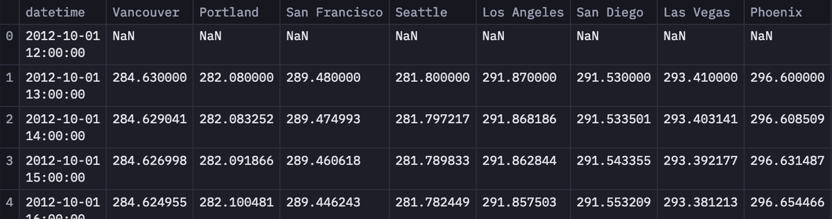

The head() method from Pandas shows the first few rows (default 5) of the data.

As you can see in the above image, the data contains the datetime column and the temperature data for different cities in individual columns.

To process the data, we will first create a list of features with the help of the following code:

column_names = [col for col in temperature_df.columns if col != "datetime"]

Next, you can use a native Hex input parameter to choose a city for the forecasting.

Once the city is selected, we need to filter the data based on that city. Also, we need to make sure that the datetime column in the dataset is in the pd.datetime() format and not in string format. Finally, for the analysis, we need to make the datetime column the index.

# Convert the 'datetime' column to datetime format
temperature_df['datetime'] = pd.to_datetime(temperature_df['datetime'])

# Select the data for New York and drop any rows with missing values
selected_temperature_df = temperature_df[['datetime', location]].dropna()

# set datetime column as the index
selected_temperature_df.set_index('datetime', inplace=True)

You might have observed that the current data is recorded hourly, for the analysis we will be resampling it to a daily basis. Also, the current temperature data is recorded in kelvins, we will be converting it to Celsius for better interpretation.

# Resample to daily frequency
selected_temperature_daily = selected_temperature_df.resample('D').mean()

selected_temperature_daily = selected_temperature_daily.reset_index()

# Rename the columns to the format expected by Prophet
selected_temperature_daily.columns = ['ds', 'y']

# Convert the temperature to Celsius for easier interpretation
selected_temperature_daily['y'] = selected_temperature_daily['y'] - 273.15

selected_temperature_daily.head()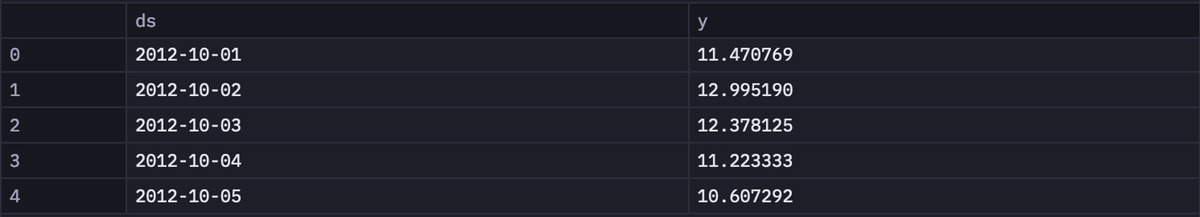

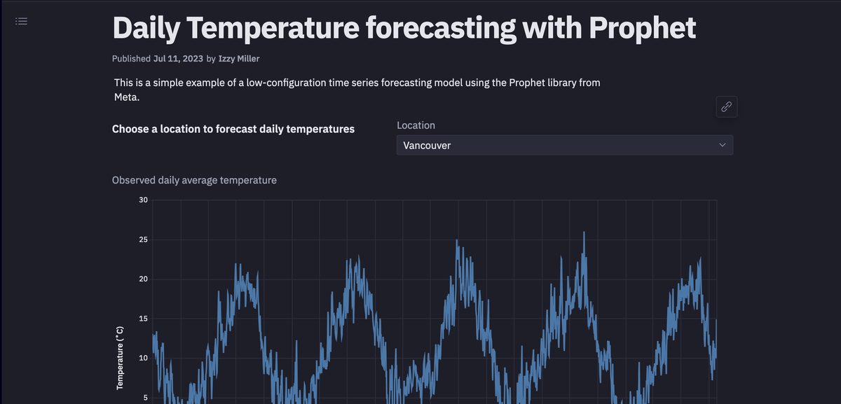
You can also use a built-in Hex chart cell to create a line plot for this time series data.

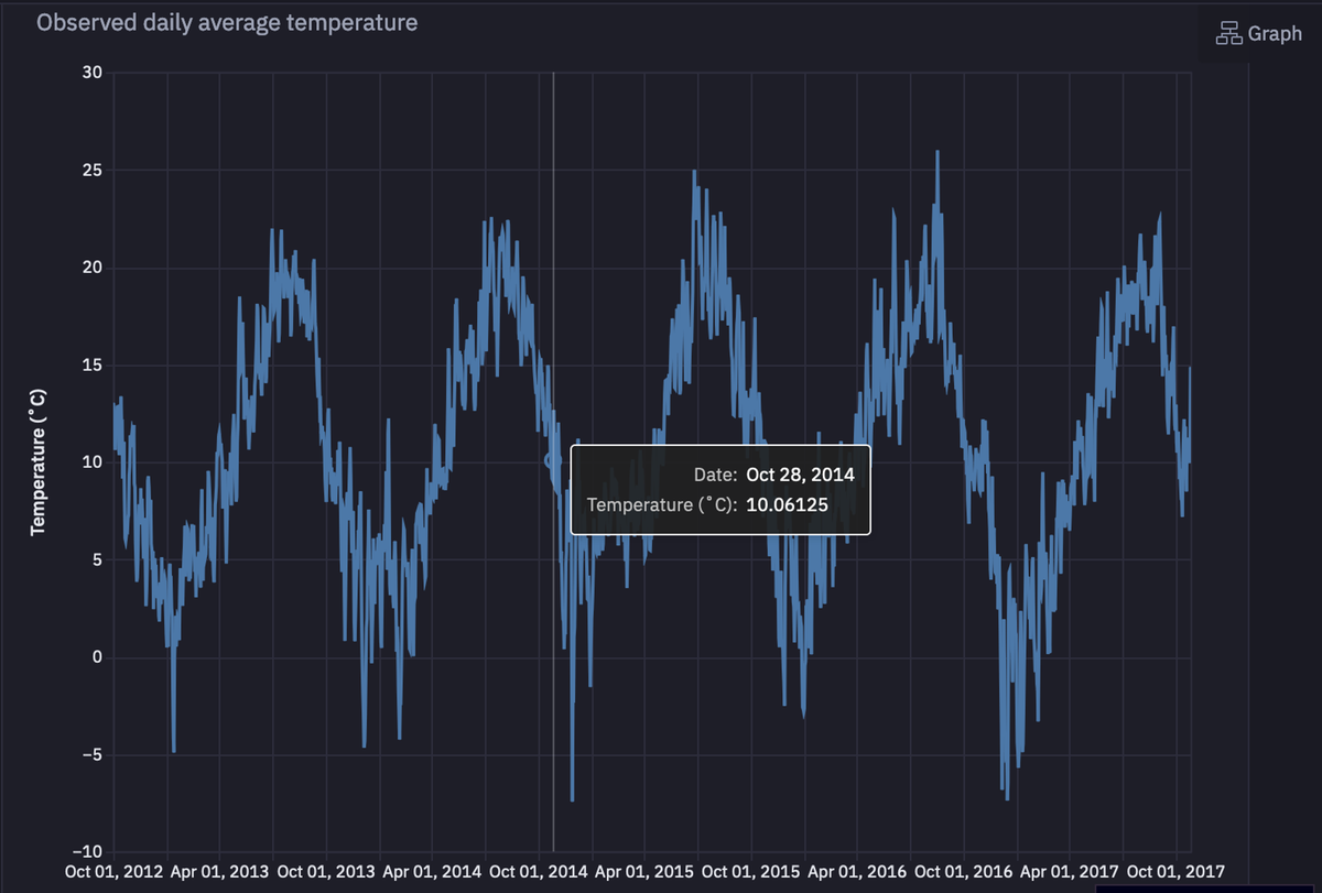
As you can see in the above image, the univariate time series data contains the seasonal patterns that occur each year.

Time Series Forecasting with Prophet

Now that your data is ready and you know about what the Prophet model is and how it works, it is time to create an object of the Prophet model and train it on the existing data using the fit()method.

# Create a Prophet instance
model = Prophet()

# Fit the model to our data
model.fit(selected_temperature_daily)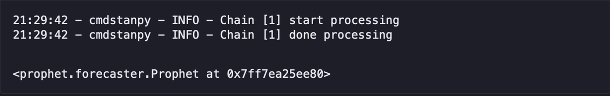

Note: The above code may take a few minutes depending on the size of data that you have.

To test the forecasting model, we will create a new dataframe that will contain the dates for the next 30 days. Once created, we will call the predict() method to get the predictions for upcoming days.

# Create a future DataFrame for the next 30 days
future = model.make_future_dataframe(periods=30, freq='D')

# Generate the forecast
forecast = model.predict(future)

forecast[['ds', 'yhat', 'yhat_lower', 'yhat_upper']].tail()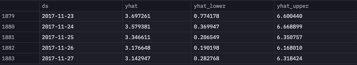

As you can see in the above image, there are three values that our prophet model returns. The yhat represents the predicted value while yhat_lower and yhat_upper represent the uncertainty intervals. These intervals can be caused by uncertainty in the trend, uncertainty in the seasonality estimates, and additional observation noise.

Note: As you might have noticed, you need not do any hyperparameter selection or tuning to train the Prophet model. This is what makes this model a lot easier to train and use.

Daily Temperature Forecast for Selected Location

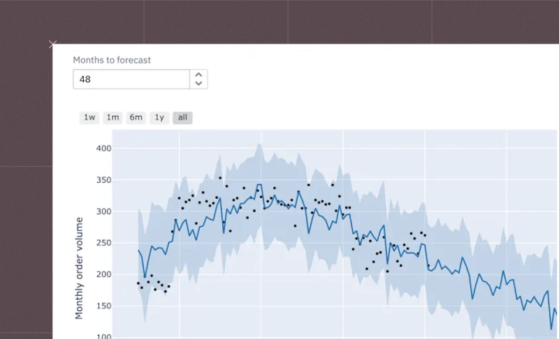
Once the model is trained and you have made predictions, you can also use a package like plotly to visualize the forecasts.

from prophet.plot import plot_plotly
import plotly.offline as pyo

fig = plot_plotly(model, forecast)
fig.update_layout(
	xaxis_title="Date",
	yaxis_title="Temperature (K)",
)
pyo.iplot(fig)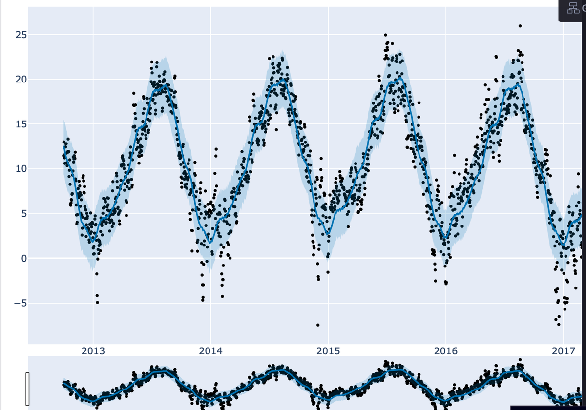

As you can observe in the above graph, the trend and seasonality are still captured in the data for future dates.

Evaluate Model Performance

There are plenty of evaluation metrics available for measuring the performance of a time series forecasting model. The most important and widely used one is the Mean Absolute Error (MAE) due to its simplicity and intuitiveness. MAE measures the absolute error between the actual values and the predicted values. Also, it does not consider the direction of the errors. The formula to calculate the MAE is as follows: MAE = (1/n) * sum(|y_true - y_pred|) where n is the number of samples, y_true is the actual samples, and y_pred is the predicted samples.

Apart from MAE, some other popular metrics are Root Mean Squared Error (RMSE), Mean Absolute Percentage Error (MAPE), Mean Absolute Scaled Error (MASE), and Symmetric Mean Absolute Percentage Error (sMAPE). To know when to use what type of metrics, you can refer to this article.

One good thing about Python language is that you need not implement everything from scratch, there are a lot of libraries that implement most of the mathematical formulas that you will need for implementation. For example, you need not implement MAE from scratch, the sklearn library already has its implementation, you just need to import it and use it with your actual samples and predicted samples as follows:

from sklearn.metrics import mean_absolute_error # Calculate the MAE for the last 365 days of the training data y_true = selected_temperature_daily['y'][-365:].values y_pred = forecast['yhat'][-365:].values mae = mean_absolute_error(y_true, y_pred)

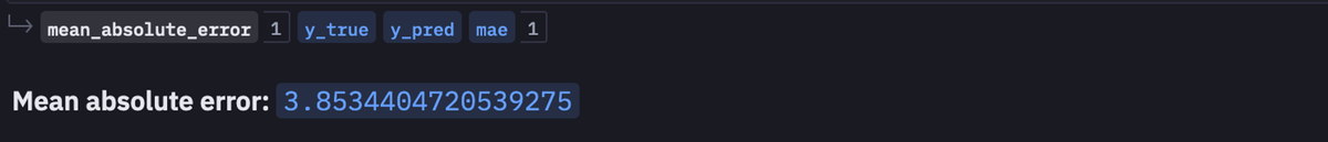
As you can see in the above image, the calculated MAE is really small which indicates that the model is trained well and can make accurate predictions.

Train Model for All Available Locations

Now that we have created a model for one of the selected locations, it is time to train the model for each location in our dataset and make predictions to compare them with one another. To do so, let’s create a Python method that iterates over each location in the dataset, applies the necessary preprocessing (that we have done earlier), trains the model, makes predictions for future dates, evaluates the model with MAE and finally compares the results of different locations.

def temperature_forecast(locations):
	most_predictable_location = None
	lowest_mae = float("inf")
	summary = []

	for location in locations:
    	selected_temperature_df = temperature_df[["datetime", location]].dropna()
    	selected_temperature_df.set_index("datetime", inplace=True)
    	selected_temperature_daily = selected_temperature_df.resample("D").mean()
    	selected_temperature_daily = selected_temperature_daily.reset_index()
    	selected_temperature_daily.columns = ["ds", "y"]
    	selected_temperature_daily["y"] = selected_temperature_daily["y"] - 273.15

    	model = Prophet()
    	model.fit(selected_temperature_daily)
    	future = model.make_future_dataframe(periods=30, freq="D")
    	forecast = model.predict(future)

    	y_true = selected_temperature_daily["y"][-365:].values
    	y_pred = forecast["yhat"][-365:].values
    	mae = mean_absolute_error(y_true, y_pred)

    	if mae < lowest_mae:
        	lowest_mae = mae
        	most_predictable_location = location

    	seasonality = forecast[["weekly", "yearly"]].abs().mean()
    	summary.append(
        	{
            	"location": location,
            	"mae": mae,
            	"weekly_seasonality": seasonality["weekly"],
            	"yearly_seasonality": seasonality["yearly"],
        	}
    	)

    	fig = model.plot(forecast)
    	plt.title(f"Temperature Forecast for {location}")
    	plt.xlabel("Date")
    	plt.ylabel("Temperature (C)")
    	plt.show()

	summary_df = pd.DataFrame(summary)
	return most_predictable_location, summary_df
    
if run_comparisons:
	locations = [col for col in temperature_df.columns if col != "datetime"]
	most_predictable, summary = temperature_forecast(locations)
	print(f"Most predictable location: {most_predictable}")
	print("Summary:")
	print(summary)

This is it, you have now created a time series forecasting model that can predict the temperature for future dates for selected locations. Once all the code part is done, you can head over to theApp section of the Hex environment and it will show you the dashboard for the code that you have written. You can customize this dashboard according to your needs by drag and drop feature.

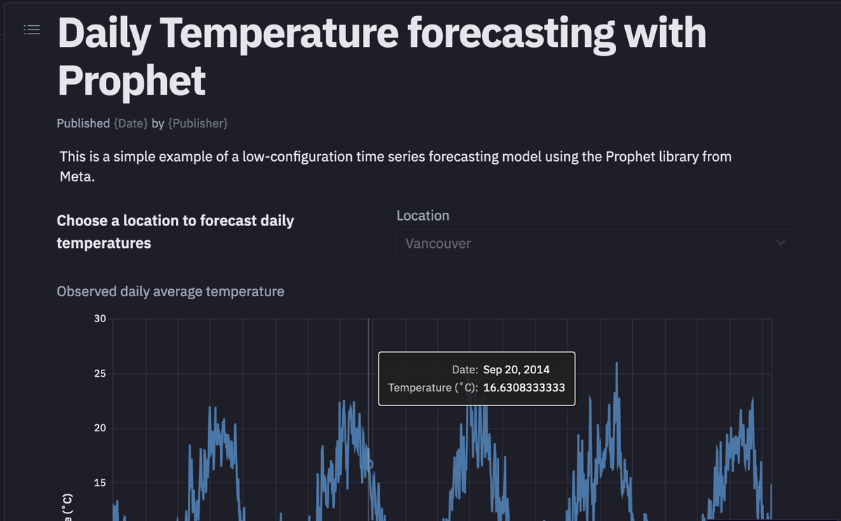
Once done, you can click on the publish button to deploy the model that you have created.

It’s really this easy to create and deploy a model in Hex!

Best Practices and Tips

Now that you have seen a practical implementation of time series forecasting it is time to discuss some of the best practices for the same.

Optimizing Model Performance

The performance of the time series model depends on the quality of data that you have. The real-world data is not suitable for the time series models almost all the time. You need to process it to make it suitable for these models. The general steps for processing include, feature engineering i.e. adding or removing features to improve the predictive performance of the model. This may include lagged variables, rolling averages, or other engineered features. Also, you must identify if input features are on the same scale, if not you need to apply the normalization and scaling techniques that can enhance the stability and convergence of the model. Apart from these, techniques like hyperparameter tuning (not for Prophet) and cross-validation help you achieve good results for your use case.

Dealing with Common Challenges in Time Series Forecasting

Some of the most common challenges in time series forecasting include the presence of outliers, the presence of missing values, and the presence of stationary components. To address the issue of missing values you must use techniques such as interpolation, forward-fill, or backward-fill. Similarly, Robust statistical methods or trimming techniques can be employed for dealing with the outliers. Additionally, both outliers and missing values require business knowledge as some of these values make sense to keep them for modeling. Finally, if your time series is non-stationary, you should apply transformations such as differencing or decomposition to make it stationary to simplify modeling.

Considerations for Deploying Prophet Models in Production

One of the important aspects of any time series forecasting model is its deployment. Sometimes use cases may require real-time inference while some use cases need batch inference. You must also serialize and save your model to load the model quickly without retraining it every time you make predictions. You must also consider the scalability of your forecasting solution especially if dealing with large datasets. Finally, your work is not completed after deployment, you must also remember the monitoring and maintenance constraints of your solution.

Navigating Time Series Challenges with Prophet and Hex

If forecasting the future was easy, everyone would be a fortune-teller. However, with the integration of Prophet and Hex, we have tools that bring us closer to accurately predicting time-based data trends. This combination enables analysts and businesses to cut through the complexities of time series data, providing clearer insights and more reliable forecasts. By using these tools, we can navigate the unpredictability of time series challenges with a level of precision and confidence that was previously unattainable, opening up new possibilities for data-driven decision-making in various industries.