Customer lifetime value Dashboard

According to the 80/20 rule from Italian economist Vilfredo Pareto, 80% of the profit of any business comes from 20% of the customers (who are regular).

As a business, you want to know who these 20% of valuable customers are. That’s where Customer Lifetime Value (CLV) analysis comes in.

CLV helps you measure the long-term value a customer brings to your business. Once you identify your most valuable customers, you can make informed decisions regarding marketing, customer acquisition, and customer retention.

This article will teach you more about this technique and how to build a CLV analysis dashboard in Python.

What is Customer Lifetime Value?

Customer lifetime value is an analytical approach that helps businesses estimate the total monetary value a customer can bring over their entire duration with the company.

To calculate CLV, businesses typically look at two key factors: the average revenue a customer generates and the average profit associated with them. Put together, these insights reveal how much a customer truly contributes to the business, beyond just a single purchase.

Why Customer Lifetime Value matters

Customer Lifetime Value (CLV) holds a lot of importance for a business due to the following reasons:

Strategic resource allocation: CLV identifies the customers with the best monetary value to the business. This helps businesses prioritize their marketing efforts and resources on the customers who generate the most revenue over the long term.

Marketing optimization: Based on CLV results, businesses tailor their marketing strategies by optimizing advertising spend, developing targeted campaigns, and creating personalized offers to attract and retain valuable customers.

Customer Segmentation: You group high CLV customers into one segment and low CLV customers into another. Then you gain insights into what works well for high CLV customers and apply those learnings to improve the CLV of others.

Optimizing Customer Acquisition Cost (CAC): By comparing CLV with Customer Acquisition Cost (CAC), businesses assess whether acquiring new customers is cost-effective or whether maintaining existing ones delivers better value.

Growth: Forecasting Revenue and CLV provides a forward-looking perspective, enabling businesses to forecast future revenue and growth. This provides valuable insights for long-term planning, supports informed strategic decision-making, and helps develop realistic and attainable corporate objectives.

These are just a few important points regarding CLV; there are, of course, many other valuable things that CLV brings to a business.

Types of Customer Lifetime Value

As mentioned, there are two primary categories of CLV: historical CLV and predictive CLV.

Historic customer lifetime value

Historical CLV measures the total revenue or profit a particular customer has generated for you to date. 

For example, if a customer continues a subscription plan of $40 per month for 12 months, you calculate the revenue as 40 × 12 = $480. This metric helps you understand your current customers, build buyer personas, or segment customers based on their spending habits. However, when used alone, it does not provide much insight into predicting future revenue.

Predictive customer lifetime value 

Predictive CLV uses machine learning and statistical techniques to estimate how long a customer continues with your business and what their total value will be. These models rely on historical data such as purchase frequency, average order value, and retention probability to estimate future value.

Businesses often use predictive CLV for planning. For example, if an e-commerce company knows the estimated number of future purchases, it can plan inventory more effectively.

How to Calculate Customer Lifetime Value

Firstly, you may calculate these metrics: 

• Average order value: the average amount a customer spends per purchase.
• Purchase frequency: the number of transactions or purchases within a specific time period. In a subscription model, this may be once a month. In e-commerce, it varies based on customer buying behavior.
• Customer lifespan: How much time a customer stays with your business.

The CLV formula looks like:

CLV = Average Order Value x Purchase Frequency x Customer Lifespan

However, you cannot directly compute CLV for new customers without any historical data. Because of this, businesses often use probabilistic models, such as the BG/NBD model, for new customers with limited history. They help fill the gap by predicting future behavior based on patterns across similar users.

Here are some popular frameworks for estimating CLV:

• Buy Till You Die (BTYD): BTYD is a framework for estimating and predicting CLV, especially for non-contractual customers. It analyzes purchasing behavior over time and assumes customers keep buying until they become inactive. The model uses probability distributions, such as the Poisson distribution for transaction counts and the Exponential distribution for inter-purchase times, to estimate the likelihood of repeat purchases. With predictive analytics, BTYD forecasts future customer behavior and estimates the expected number of purchases from each customer.
• BG/NBD Model: The Beta Geometric/Negative Binomial Distribution (BG/NBD) is one of the most widely used models in customer analytics for churn and CLV estimation. It combines the Beta distribution and the Negative Binomial distribution to capture customer behavior. The model predicts the probability that a customer becomes inactive and estimates the distribution of transactions made by active customers.
• Gamma-Gamma Model: The Gamma-Gamma model focuses on estimating the monetary value or average transaction size of customers in non-contractual settings. It relies on the Gamma distribution and often works alongside the BG/NBD model to enhance CLV analysis. The model considers two factors: how often a customer transacts and how much money they spend per transaction. This makes it especially useful in businesses where spending habits vary significantly among customers.
• Predictive Modeling: In non-contractual or non-subscription settings, predictive models help when the dataset includes new customers with limited history. These approaches use machine learning algorithms such as clustering, classification, and regression, depending on the use case. Predictive modeling identifies patterns in existing data and applies them to forecast the potential lifetime value of customers with less historical information.

Implementing CLV in Python and Hex

Now that you know the methods for calculating CLV, it’s time to put them to work on real data. In this section, you build a live dashboard on Hex.

Hex is an interactive analytics workspace where you write and run code in a single, shareable environment. You mix SQL, Python, and R in separate cells, run and debug code easily, and create no-code visualizations that turn results into clear, interactive charts. Hex connects directly to databases and cloud data stores, making data import and export feel straightforward rather than painful.

For our setup, we use Python 3.11 on Hex and install dependencies with pip. The dataset comes from an online retail store and lives in a Snowflake warehouse.

Install and Load Dependencies

To begin with, let’s install all the necessary Python dependencies with the help of PIP as follows:

$ pip install pandas numpy
$ pip install Lifetimes

The Pandas and Numpy libraries will be used for manipulating data, and the Lifetimes library will be used to perform different CLV algorithms, as it implements all of them.

Once installed, you can import the dependencies in the Hex environment as follows:

import lifetimes
import pandas as pd
import numpy as np
from lifetimes import BetaGeoFitter
from lifetimes import GammaGammaFitter

Load and explore the data

Our data is stored in a Snowflake warehouse, and we can easily read it into the Hex environment with the help of a simple SQL statement. The data is always loaded into a Pandas DataFrame, which makes the data processing and manipulation a lot easier.

select * from "DEMO_DATA"."DEMOS"."ONLINE_RETAIL"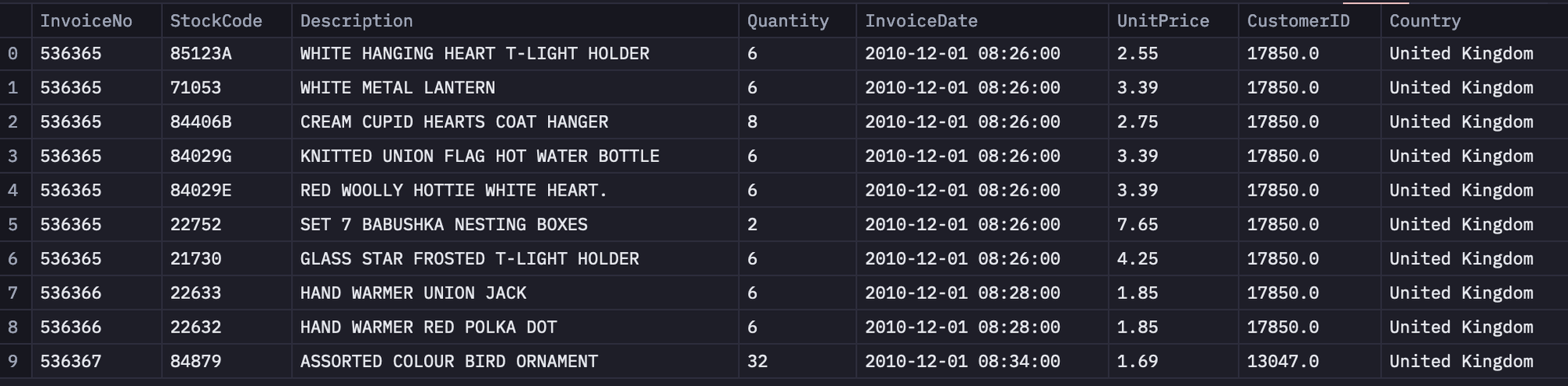

Next, we will use some built-in Python methods to understand the data. Let’s begin with checking the descriptive statistics of all the numerical features in the dataset using the `describe()` method from Pandas.

df.describe()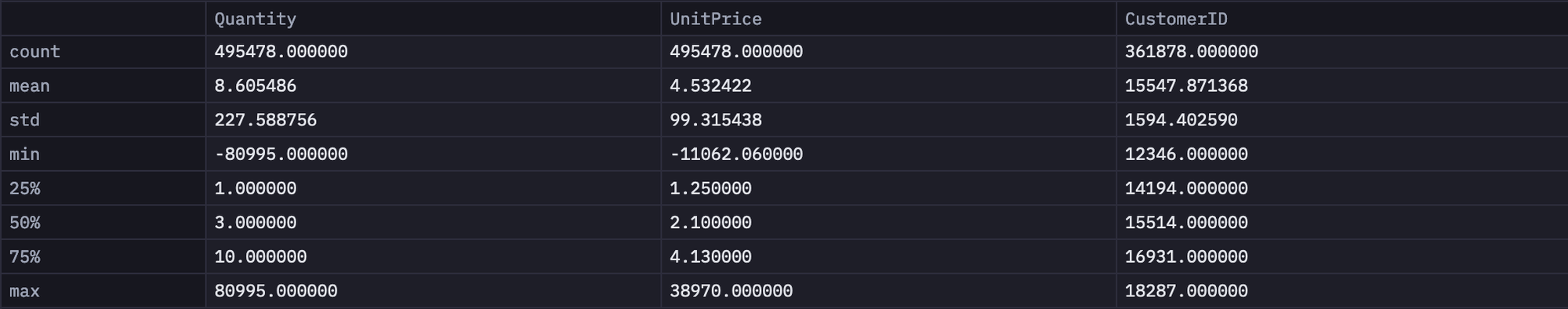

As you can see in the above image, the `Quantity` and `UnitPrice` columns have a really small value for mean, while their min and max values are quite extreme. This shows the presence of outliers in the dataset.

Next, we will check the presence of NaN (Null) values in the dataset. To do so, you can use the `install ()` method to get all the null values in a column and the `sum()` method to get an aggregate sum for the same.

df.isnull().sum()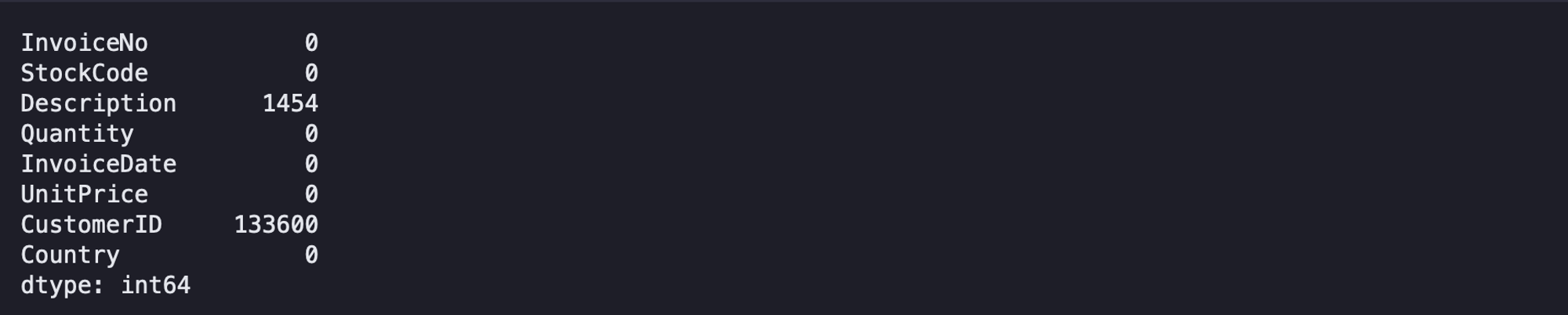

The `CustomerID` and `Description` columns contain some NaN values that we will have to remove to proceed with CLV analysis.

Data cleaning

As part of data cleaning, we will address the outliers and the null values in the dataset.

• Keep only the rows where at least one order is placed with a valid quantity greater than 0.
• Remove items that have a cost less than or equal to 0, since they don’t contribute to revenue.
• Exclude all returned orders from the dataset.
• Drop rows with null values, as the dataset already has plenty of valid records.
• Convert the `CustomerID` field from float to string for consistency.
• Strip the time component from the `InvoiceDate` field and keep only the date.

All these changes can be made using dataframe filtering and basic Pandas functions as follows:

df = df[df['Quantity'] > 0 ] # takes care of unaccounted returns or cancellations
df = df[df['UnitPrice'] > 0] # remove items that appear not to cost anything
df = df[~df['InvoiceNo'].str.contains("C",na=False)] # drop returned items
df.dropna(inplace=True) # drop all nulls
df['CustomerID'] = df['CustomerID'].astype(str) # convert customerID to a string
df["InvoiceDate"] = pd.to_datetime(df["InvoiceDate"]).dt.date # removes time component from date

Next, we will create a Python function for detecting the outliers using the Interquartile range. All the values that fall below Q1 and above Q3 are considered outliers. So we will create a method to calculate the lower (Q1) and upper (Q3) limits of our data.

def outliers(values):
	# Calculate the 5th and 95th percentiles of the input values
	q1, q3 = np.percentile(values, [5, 95])

	# Calculate the interquartile range (IQR)
	iqr = q3 - q1

	# Calculate the lower and upper outlier limit
	lower = q1 - (1.5 * iqr)
	upper = q3 + (1.5 * iqr)
	return lower, upper

Finally, we will create another Python method that takes a dataframe feature, calculates the lower and upper limits for that feature, and then filters the values that fall beyond these limits.

def remove_outliers(frame, column):
	# Calculate the lower and upper outlier limit for the specified column
	lower, upper = outliers(frame[column])

	# Create filters that remove all rows that fall outside of these limits
	lower_mask = frame[column] > lower
	upper_mask = frame[column] < upper

	# Apply the filters to the dataset
	cleaned_frame = frame[lower_mask & upper_mask]
	return cleaned_frame

Since outliers are present in the `Quantity` and `UnitPrice`, we will apply the above method to these columns.

data = remove_outliers(df, 'Quantity')
data = remove_outliers(data, 'UnitPrice')

Once the outliers are removed, we can check the descriptive statistics of the data again.

data.describe()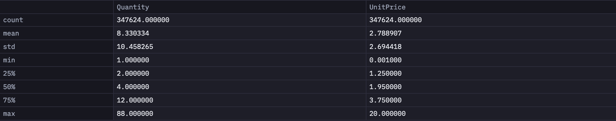

You can notice in the above image that the outliers are removed, as there are no extreme values present in any of these features.

Next, we will create an extra column `TotalPrice` that will be the result of the multiplication of `UnitPrice` and `Quantity`.

data['TotalPrice'] = data['UnitPrice'] * data['Quantity']

Before applying any CLV analysis method, we will first check the total number of unique customers and the total revenue earned from all orders made.

customers = data['CustomerID'].nunique()
revenue = data['TotalPrice'].sum()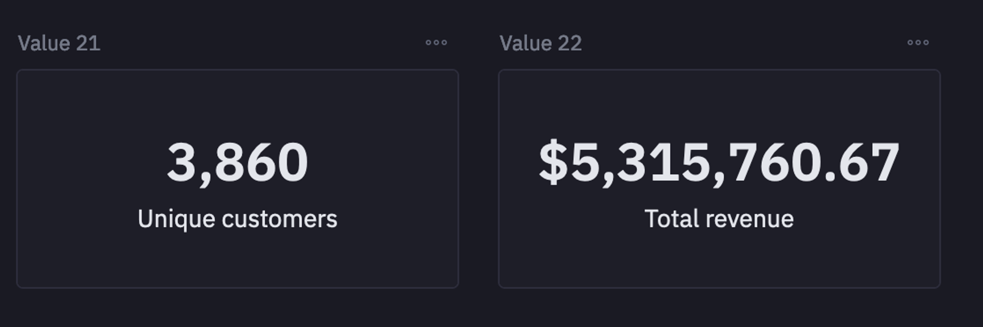

Buy till you die model

Now that you have a clean dataset and understand the information it contains, it’s time to move into the analysis. 

In this section, we use the BG/NBD and Gamma-Gamma models to estimate customer lifetime value. 

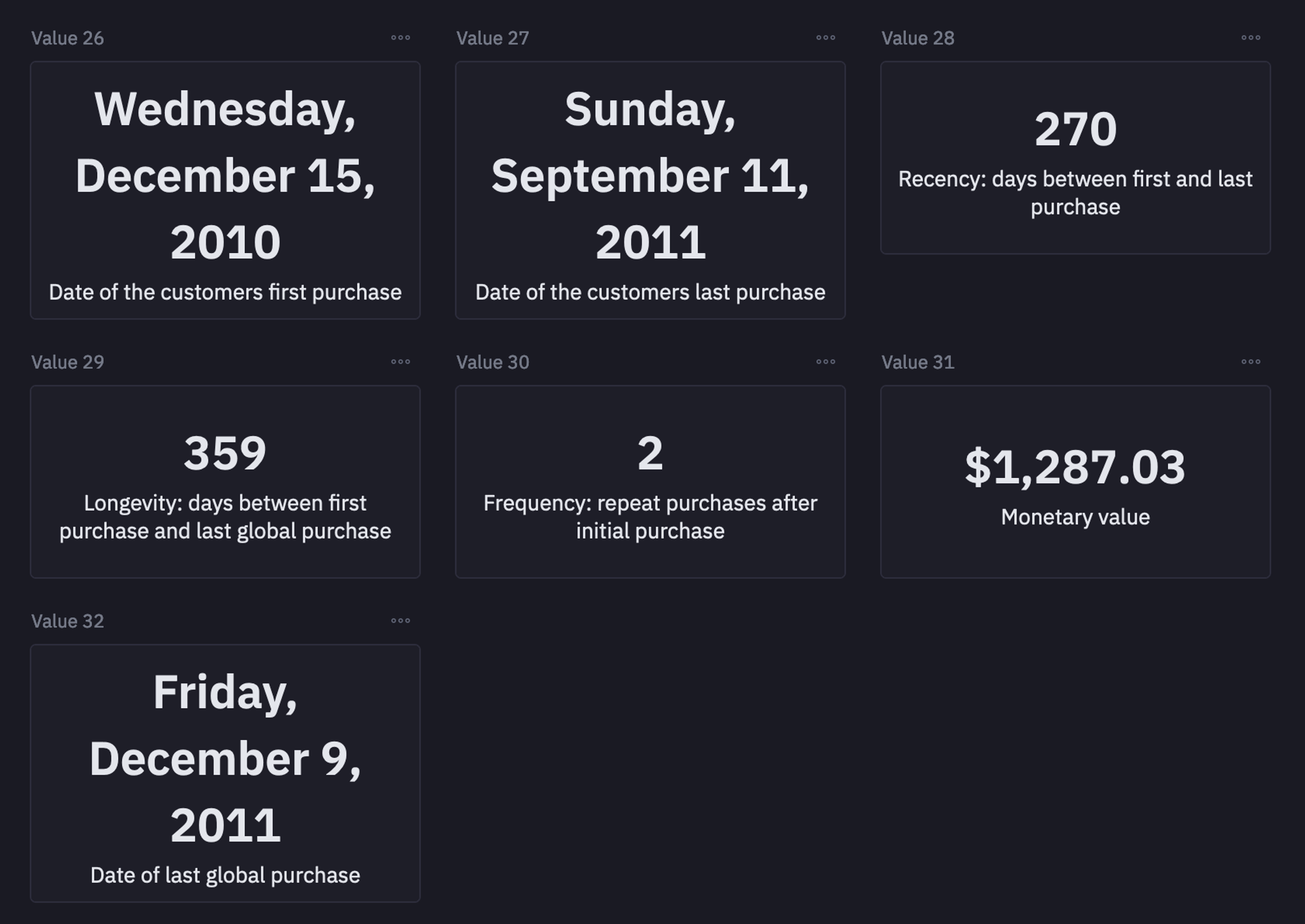
To illustrate the process, we select a single customer from the dataset and calculate all the key metrics (outlined in the previous section) for that customer.

if cust:
	# Select a random customer from the dataset
	customer = np.random.choice(data["CustomerID"])
else: customer = '13124.0'

# Filter the dataset to only include data for the selected customer
customer_data = data[data["CustomerID"] == customer]

# Find the date of the customer's first purchase
birth = customer_data["InvoiceDate"].min()

# Find the date of the customer's most recent purchase
latest = customer_data["InvoiceDate"].max()

# Find the date of the most recent purchase in the entire dataset
last_global_purchase = data["InvoiceDate"].max()

# Calculate the customer's CLV (Customer Lifetime Value) summary data
customer_clv = lifetimes.utils.summary_data_from_transaction_data(
	customer_data,
	"CustomerID",
	"InvoiceDate",
	"TotalPrice",
	observation_period_end=last_global_purchase,
)

# Extract the recency value from the CLV summary data
recency = customer_clv["recency"][0]

# Extract the frequency value from the CLV summary data
frequency = customer_clv["frequency"][0]

# Extract the longevity value (time since first purchase) from the CLV summary data
longevity = customer_clv["T"][0]

# Extract the monetary value from the CLV summary data
monetary_value = customer_clv["monetary_value"][0]

As you can see in the above code chunk, we are first extracting the birth date, the date of the customer’s first purchase, the date of the customer’s most recent purchase, and the date of the most recent purchase in the entire dataset. 

Then we pass the required details such as `CustomerID`, `InvoiceDate`, `TotalPrice`, and `last_global_purchase`, into the `summary_data_from_transaction_data()` method from `lifetime.utils`. This generates the CLV summary for the selected customer.

To apply this for all the customers, we need to call the `summary_data_from_transaction_data()` method over the entire dataset.

clv = lifetimes.utils.summary_data_from_transaction_data(data,'CustomerID','InvoiceDate','TotalPrice',observation_period_end='2011-12-09')
clv = clv[clv['frequency']>1] # We want only customers who've shopped more than 2 times

This is it, you now have a new dataframe (clv) that will be used further for analysis.

BG/NBD model for predicting the purchase frequency

Now we use the BetaGeoFitter to apply the BG/NBD model to the newly created dataframe. This model predicts the number of purchases each customer is likely to make within a defined time period.

bgf = BetaGeoFitter(penalizer_coef=0.001)
bgf.fit(clv['frequency'], clv['recency'], clv['T'])

Once you have trained the model, you can choose the number of months to look into the future. This is where you can use the feature from Hex to define a slider to select the number of months (eg, 8).

After selecting the number of months, you can use the `conditional_expected_number_of_purchases_up_to_time()` method to predict the number of purchases for the defined months.

t = months * 30 # 30 day period
clv['expected_number_of_purchases'] = bgf.conditional_expected_number_of_purchases_up_to_time(t, clv['frequency'], clv['recency'], clv['T'])
clv.sort_values(by='expected_number_of_purchases',ascending=False).head(5)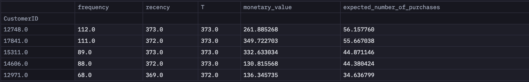

Gamma - Gamma Model

Finally, we will implement the Gamma-Gamma model to estimate how much a customer is likely to spend on average in future purchases.

The Gamma-Gamma model assumes that there is no correlation between the monetary value and the purchase frequency. 

This means that the amount spent on purchase does not directly depend on the number of times the customer visits the store. To check the correlation between these two features, you can use the `corr()` method.

clv[['frequency','monetary_value']].corr()

Since no correlation can be seen between these two columns, we are good to go with the Gamma-Gamma model. To apply this model, you can use the following code:

gf = GammaGammaFitter(penalizer_coef=0.01)
ggf.fit(clv["frequency"],
    	clv["monetary_value"])

Customer Lifetime Value for selected months

We will use these trained models (Gamma-Gamma and BG/NBD) to calculate the CLV for each customer. We can calculate the CLV for the selected number of months as follows:

lifetime_value = clv.copy()
lifetime_value["Lifetime_value"] = ggf.customer_lifetime_value(
	bgf,
	lifetime_value["frequency"],
	lifetime_value["recency"],
	lifetime_value["T"],
	lifetime_value["monetary_value"],
	time = months,
	freq="D",
	discount_rate=0.01,
)

Finally, to check the calculated values, you can use the following line of code:

lifetime_value[['monetary_value', 'expected_number_of_purchases', 'Lifetime_value']].sort_values('Lifetime_value',ascending=False).head()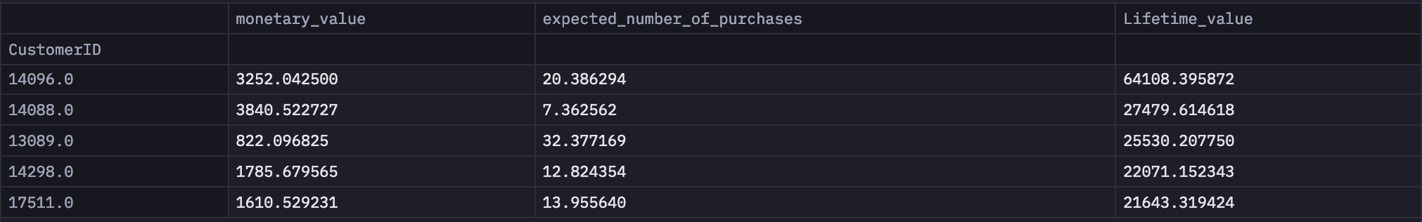

Customer segmentation for selected months

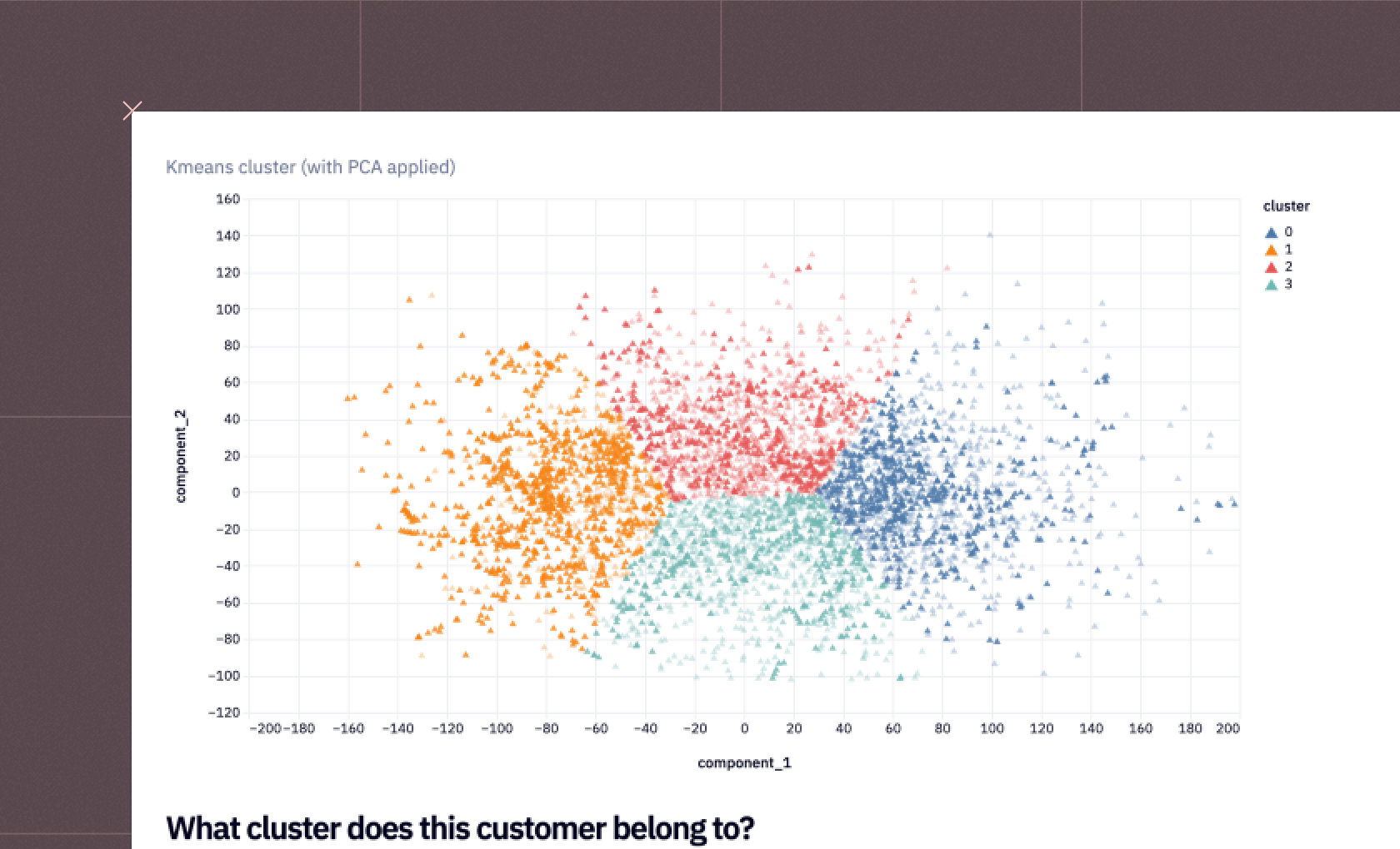
You can also segregate the customers into four different groups i.e. “Hibernating”, “Need Attention”, “Loyal Customers”, and “Champions” (arranged from least valuable to the most) based on their N-month (eg. 6-month) Customer Lifetime Value (CLV).

lifetime_value["Segment"] = pd.qcut(
    lifetime_value["Lifetime_value"],      # The CLV data to be divided into quartiles
    4,                                     # Number of equal groups (quartiles)
    labels=[
        "Hibernating",                     # Lowest quartile (bottom 25%)
        "Need Attention",                  # Second quartile (25-50%)
        "Loyal Customers",                 # Third quartile (50-75%)
        "Champions"                        # Highest quartile (top 25%)
    ]
)

To check the segments for the customers, you can use the following line of code:

lifetime_value[['expected_number_of_purchases', 'Lifetime_value', 'Segment']].sort_values('Lifetime_value',ascending=False).head()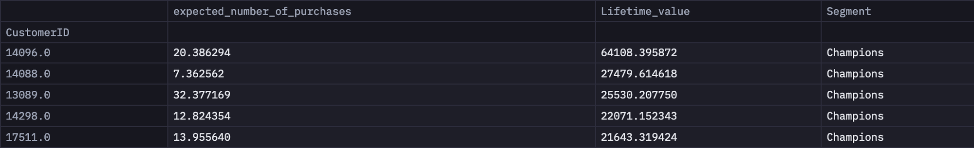

Group by segment for the next selected months

You can also calculate an aggregate across all the categories in the data to get an overall picture. You can do so with the help of the following SQL command:

SELECT
	Segment,
	AVG("T") AS "T",
	AVG(recency) AS recency,
	AVG(frequency) AS frequency,
	AVG("Lifetime_value") as "Lifetime_value", AVG(monetary_value) as monetary_value, AVG(expected_number_of_purchases) as expected_number_of_purchases
FROM lifetime_value
GROUP BY Segment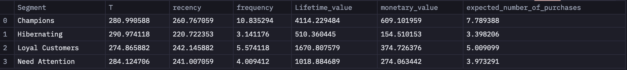

Finally, to check the average lifetime value across different customer segments, you can use the following code:

segment_stats['Lifetime_value'] = segment_stats[['Lifetime_value']].apply(lambda x: round(x, 2))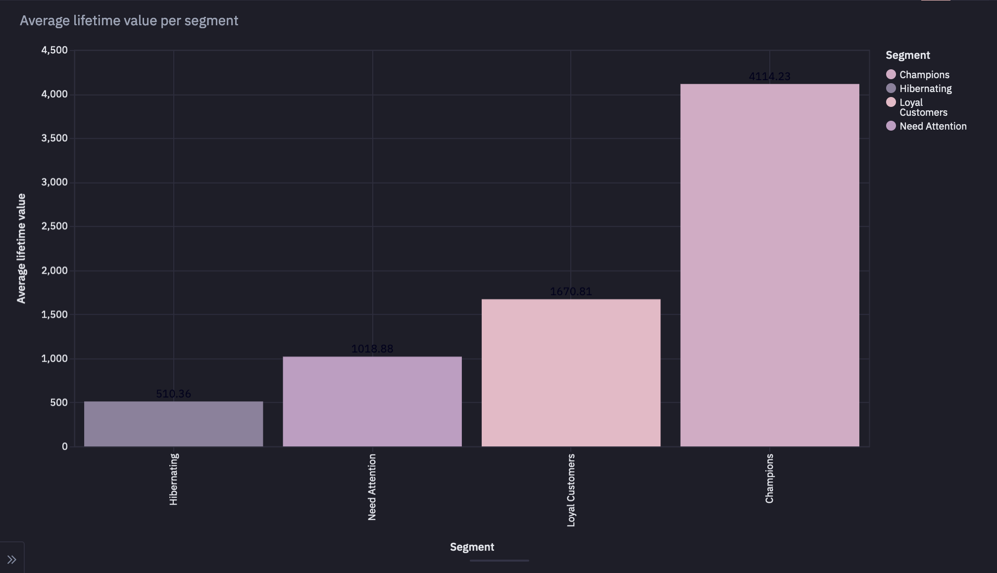

As you can see in the above graph, the dataset contains a larger number of champions as compared to other categories.

This is it, you have now created your dashboard for Customer Lifetime Value Analysis using Python and Hex. 

How to increase customer lifetime value

Understanding CLV is one thing, but the real impact comes from knowing how to grow it. Let’s dive into the strategies businesses use to increase customer lifetime value and turn one-time buyers into long-term loyalists.

Collect and act on feedback

Feedback is fuel for growth. The more specific and detailed it is, the more useful it becomes. Start by focusing on your revenue-driving customers. Set up interviews to dig into their experiences and capture feedback you can actually act on. 

This helps you prioritize the areas of your business that directly influence both customer satisfaction and revenue growth. Just as necessary, make sure you also collect insights on what they already love, so you can keep delivering it consistently.

For your broader customer base, use survey forms to gather Net Promoter Score (NPS) data. NPS gives you insights into overall customer satisfaction and loyalty trends.

Customer service

A Capgemini survey found that 8 out of 10 customers are willing to pay more for better service quality. Delivering consistent, high-quality support not only creates happier experiences but also strengthens loyalty and retention.

If you haven’t already, here are a few steps worth implementing:

• Provide 24/7 support.
• Offer priority or dedicated support for premium and enterprise clients.
• Enable live chat support for quick resolutions.
• Build clear, actionable documentation and resources to answer common questions.

Encourage long-term contracts

The length of time a customer stays with you has a direct impact on CLV. The longer the relationship, the higher the value.

If you run a subscription-based business, one way to extend customer lifespan is by offering discounts on annual plans. Encouraging customers to switch from monthly to annual subscriptions locks in commitment for a longer period and naturally boosts CLV.

Run loyalty programs

Loyalty programs are another proven way to keep customers coming back. Small gestures like offering a coupon for the next purchase create repeat business and reinforce customer habits. 

For a more substantial impact, design structured loyalty plans that go beyond discounts. Offer perks such as free delivery, exclusive deals, or early access to new products. Customers who enroll in these programs often remain longer and engage more deeply with your brand.

A great example is Amazon Prime. Members not only get free and fast delivery, but also access to music, movies, and other services. By bundling multiple benefits, Amazon ensures customers stay within its ecosystem for a variety of needs, increasing both retention and overall lifetime value.

Conclusion

Customer Lifetime Value is a guide for building sustainable growth. By analyzing recency, frequency, monetary value, and customer age, you uncover buying patterns that help you segment customers and design more innovative strategies.

Whether it’s improving customer service, acting on feedback, running loyalty programs, or encouraging long-term contracts, each step you take to raise CLV directly boosts retention and revenue. With tools like Python and Hex, you can model CLV, visualize it, and turn insights into action.

Ready to build your Customer Lifetime Value analysis? Sign up for Hex today and get started.