Outlier Detection

Outliers are a simple concept— data points that stand out from the rest of the data in a dataset. But identifying outliers can have an outsize importance, because outliers can seriously distort data analysis and predictions if not addressed. Detecting (and addresing) outliers helps ensure that our conclusions and decisions are based on accurate and reliable data.

A few examples of outlier detection in different industries:

• Fraud Detection: Imagine a credit card company. Outlier detection can help identify unusual spending patterns, like a sudden surge in charges from a different country, which might indicate fraudulent activity.

• Medical Diagnosis: In healthcare, outliers in blood test results could signal potential health problems that need further investigation.

• Network Security: Outlier detection can be used to monitor network traffic and identify suspicious activity, like a sudden spike in data transfer that might indicate a cyberattack.

• Equipment Maintenance: Machine sensors can detect unusual vibrations or temperature changes. Outlier detection can help identify these anomalies and prevent equipment failures.

• Scientific Discovery: Sometimes, outliers can be exciting! In science, outliers might lead to discoveries that challenge existing theories.

In this article, you'll gain a solid understanding of outlier detection with Python and Hex. You'll explore real-world applications, uncover different types of outliers, and dive into common methods for identifying them. You'll even see some best practices to ensure your analysis is accurate and effective!

Types of Outliers

There are several types of outliers, and each has unique traits and ramifications. For efficient outlier detection and data analysis, it is imperative to comprehend the many forms of outliers.

Global Outliers

Extreme values that drastically differ from the remainder of the dataset in all attributes or dimensions are referred to as global outliers. Errors in measurement, data entry, or infrequent occurrences can all cause them. For instance, the extremely high compensation of a CEO might be seen as a worldwide outlier in a dataset of staff pay.

Contextual Outliers

When examining a dataset as a whole, data points that are unique within a particular context or subgroup are contextual outliers. But they may represent some significant information due to which sometimes they may not be regarded as outliers. To recognize these outliers, you frequently need to have a deeper understanding of the context or the topic. For example, in a customer transaction dataset, a significant purchase amount might be typical for high-net-worth individuals as compared to the general public.

Collective Outliers

These outliers take the form of collections or clusters of data points that, when taken as a whole, show peculiar behavior. Even though every one of the cluster's data points might not be an outlier on its own, the cluster's overall behavior differs from the rest of the dataset. In time series data anomaly detection, network traffic analysis, and spatial data analysis, collective outliers are frequently encountered.

Common Methods for Outlier Detection

In the realm of outlier detection, various methods are employed to identify and flag data points that deviate significantly from the norm. These methods play a crucial role in ensuring the integrity and accuracy of data analysis and modeling processes.

• Statistical Methods. Statistical methods for outlier detection rely on mathematical principles to identify data points that lie outside the expected range of values. These methods are particularly useful for detecting outliers in normally distributed datasets and are widely employed across various domains for their simplicity and effectiveness.

• Z-score: The Z-score method measures how many standard deviations a specific data point is away from the mean. A standard deviation is a measure of how spread out the data is. A higher Z-score indicates that the data point is further from the mean, suggesting it may be an outlier. The formula for calculating the Z-score is: z = (x – μ) / σ. Where X is the value of the data point, μ is the mean of the dataset, and σ is the standard deviation.

• Modified Z-Score: The Z-score method can be sensitive to extreme outliers. Modified Z-score addresses this by replacing very high or low values with values closer to the central tendency (mean or median) before calculating standard deviations and Z-scores. This helps to reduce the influence of extreme outliers on the overall spread of the data. It replaces the standard deviation with the median absolute deviation (MAD) to reduce the influence of extreme values on the calculation.

• Interquartile Range (IQR): The interquartile range (IQR) method identifies outliers based on the spread of the middle 50% of the data. It calculates the range between the first quartile (Q1) and the third quartile (Q3) and considers data points outside a certain range from the quartiles as outliers. IQR is a robust method that works well with skewed or non-normal data.

• Distance-Based Methods: Distance-based methods for outlier detection focus on measuring the distance between data points in a dataset to identify outliers. These methods are particularly effective in detecting outliers in high-dimensional datasets or datasets with complex structures. By calculating distances between data points, these methods can identify outliers based on their proximity to other data points, clustering patterns, or density variations. Distance-based methods are commonly used in scenarios where traditional statistical methods may not be suitable, such as in datasets with non-normal distributions or datasets with mixed types of variables.

• DBSCAN (Density-Based Spatial Clustering of Applications with Noise): DBSCAN is a density-based clustering algorithm that identifies clusters of data points based on their density. It classifies data points into three categories: core points, border points, and noise points (outliers). DBSCAN defines clusters as areas of high density separated by areas of low density. Outliers are identified as data points that do not belong to any cluster or fall within Low-density Regions. The key parameters of DBSCAN are the minimum number of points required to form a cluster (minimum points) and the maximum distance threshold (EPS) that defines the neighborhood of a point.

• HBOS (Histogram-based Outlier Score): HBOS is an unsupervised outlier detection algorithm that computes an outlier score for each data point based on its deviation from the typical behavior observed in the dataset. HBOS constructs histograms to approximate the distribution of each feature in the dataset. It then computes the likelihood of a data point being an outlier based on its values across multiple features. HBOS is particularly efficient for high-dimensional datasets and is less sensitive to parameter tuning compared to other outlier detection methods. It is often used in scenarios where the underlying data distribution is not well understood or when the dataset contains mixed types of variables.

• Machine Learning Methods. Machine learning methods offer powerful tools for outlier detection, especially when dealing with complex data patterns or high-dimensional datasets. These methods can learn the underlying structure of "normal" data and then identify points that deviate significantly from that structure. Here's a breakdown of some popular machine-learning techniques for outlier detection:

  • Isolation Forest: Isolation Forest is a tree-based anomaly detection algorithm that isolates outliers by randomly selecting features and splitting data points into partitions. Outliers are expected to have shorter path lengths in the resulting trees compared to normal data points, making them easier to isolate. Isolation Forest is particularly efficient for high-dimensional datasets and is less sensitive to the presence of irrelevant features.

  • One-Class SVM (Support Vector Machine): SVMs are traditionally used for classification, but one-Class SVMs are a clever adaptation for outlier detection. They learn a boundary around the "normal" data in the training process. Points that fall outside this boundary are flagged as potential outliers. One-class SVMs are effective for high-dimensional data where defining clear separation lines between classes might be challenging.

  • Elliptic Envelope: Elliptic envelope method assumes the normal data follows an elliptical distribution (like a stretched circle). It estimates the parameters of this ellipse and identifies points that fall far outside the ellipse as outliers. The Elliptic Envelope is a good choice when your data exhibits an elliptical or elongated cluster pattern.

  • Autoencoder: Autoencoder is a type of neural network architecture used for unsupervised learning tasks, including outlier detection. It learns to reconstruct input data points by encoding them into a lower-dimensional representation and then decoding them back to their original form. Outliers are identified as data points that cannot be accurately reconstructed by the autoencoder model. Autoencoder-based outlier detection is effective in capturing complex data patterns and can adapt to various types of data distributions.

Outlier Detection with Python and Hex

Now that you know about outliers and the importance of detecting them, it is time to see the practical implementation with Python and Hex. Hex is a modern data platform for data science and analytics, that gives you a notebook-based workspace for developing models of any kind— including collaborative filtering models. Hex is a polyglot platform that allows you to write code in different languages within the same development environment. It can connect to various data sources including different databases, data warehouses, and cloud storage. It also provides easy visualization with the help of its no-code cells.

With Hex, you can easily integrate Python's Scikit-learn, use IQR techniques, or apply Z-scores to pinpoint outliers. Streamline your data analysis, ensure quality, and drive accurate results by efficiently identifying and addressing these deviations.

For this article, we will be generating a sample dataset to identify outliers within that, you will also see a clear explanation of the methodology employed.

Let's dive in!

Install and Load Dependencies

To implement outlier detection, you need a set of Python dependencies that can load and preprocess the data, provide visualization features, and finally libraries that provide the implementation of various statistical methods. Although Hex comes up with a lot of libraries preinstalled, you can install the libraries with the help of PIP if needed. Use the following command to install the necessary requirements:

To implement outlier detection, you need a set of Python dependencies that can load and preprocess the data, provide visualization features, and finally libraries that provide the implementation of various statistical methods. Although Hex comes up with a lot of libraries preinstalled, you can install the libraries with the help of PIP if needed. Use the following command to install the necessary requirements:

$ pip install pandas
$ pip install numpy
$ pip install matplotlib, seaborn
$ pip install scikit-learn

Once the dependencies are installed, you can load them in the Hex environment as follows:

import numpy as np
import pandas as pd
import matplotlib.pyplot as plt
import seaborn as sns
from sklearn.ensemble import IsolationForest
from sklearn.metrics import precision_score, recall_score, f1_score

The numpy and pandas libraries will help us load and preprocess the data, the matplotlib and seaborn libraries will help us create the visualizations, and the sklearn library will help us implement and assess the outlier detection algorithm.

Generate Sample Dataset

We'll generate a dataset with two numerical features. Each feature will be normally distributed, but we'll add a few outliers to each one. We'll label these outliers so we can evaluate our outlier detection algorithm's performance later. To do so, we will be using the random.normal() method from Python as follows:

# Set a random seed for reproducibility
np.random.seed(42)

# Generate normally distributed data
data = np.random.normal(size=(1000, 2))

# Introduce outliers into the data
outliers = np.random.uniform(low=-10, high=10, size=(50, 2))

# Combine the data
combined_data = np.vstack([data, outliers])

# Create a binary label indicating whether each point is an outlier
labels = np.zeros(1050)
labels[1000:] = 1  # The last 50 points are outliers

# Create a DataFrame from the data
df = pd.DataFrame(combined_data, columns=['Feature 1', 'Feature 2'])
df['Outlier'] = labels

df.head()

In the above code, we started with setting the seed with random.seed() method from numpy that allows us to generate the same values (reproducibility) every time we run the code. Then, the random.normal() method generated the 1000 normally distributed data points, and using the random.uniform() method, we generated some outliers to add to this normally distributed data. Next, we combined the normally distributed data and outliers with the help of the vstack() command. Then we created a new variable named labels that will indicate the outliers i.e. the first 1000 data points will have a corresponding value 1 indicating no outlier while the rest of the values for the label are 0 indicating outliers. Finally, we created a dataframe to store this normally distributed and outlier data.

Visualize the Data

As a next step, let's visualize this dataset to understand what the outliers look like for this case. Plotting data is a great way to get a sense of what we're dealing with. We'll color-code the points based on whether they're outliers or not. Scatter plots are the primary choice for visualizing the outliers, that is why we will use the scatterplot() method from Seaborn.

# Set the style of the plot
sns.set_style('whitegrid')

# Create a scatter plot
plt.figure(figsize=(10, 8))
sns.scatterplot(x='Feature 1', y='Feature 2', hue='Outlier', data=df, palette='Set1', alpha=0.8)

# Add title and labels
plt.title('Scatter Plot of the Data', fontsize=16)
plt.xlabel('Feature 1', fontsize=14)
plt.ylabel('Feature 2', fontsize=14)

plt.show()

In the above code, we first decided on the plot style as whitegrid, then we used the figure() method from matplotlib to set the figure size. Then we created a scatter plot using the scatterplot() method. Finally, we have added some explanatory details like labels and titles to the plot.

Outlier Detection

Now, let's move on to the main event: outlier detection. We'll use a technique called the Isolation Forest, which is a type of ensemble learning method. It is particularly good at dealing with high-dimensional data and is relatively efficient.

Sklearn library in Python provides the implementation of the Isolation Forest. You can apply it to this manually created data as follows:

# Initialize the Isolation Forest model
clf = IsolationForest(contamination=0.05, random_state=42)

# Fit the model
clf.fit(df[['Feature 1', 'Feature 2']])

# Predict the outliers in the data
df['Predicted Outlier'] = clf.predict(df[['Feature 1', 'Feature 2']])
df['Predicted Outlier'] = df['Predicted Outlier'].map({1: 0, -1: 1})

df.head()

In the above code, we have created an object of Isolation Forest using the IsolationForest() method. Then we trained this model on our dataset using the fit() method. Finally, we have used the predict() method to predict the outliers and stored the results in the original dataframe under the Predicted Outlier column.

Evaluate the Model

Since we have our ground truth data as well as predicted data, we can use any classification metrics like accuracy, precision, recall, etc. to assess the performance of the Isolation Forest model. The best part is, sklearn also provides the implementation of these performance metrics. To calculate the precision, recall, and F1-score for our data following lines of code can be used:

# Calculate precision, recall, and F1 score
precision = precision_score(df['Outlier'], df['Predicted Outlier'])
recall = recall_score(df['Outlier'], df['Predicted Outlier'])
f1 = f1_score(df['Outlier'], df['Predicted Outlier'])

precision, recall, f1

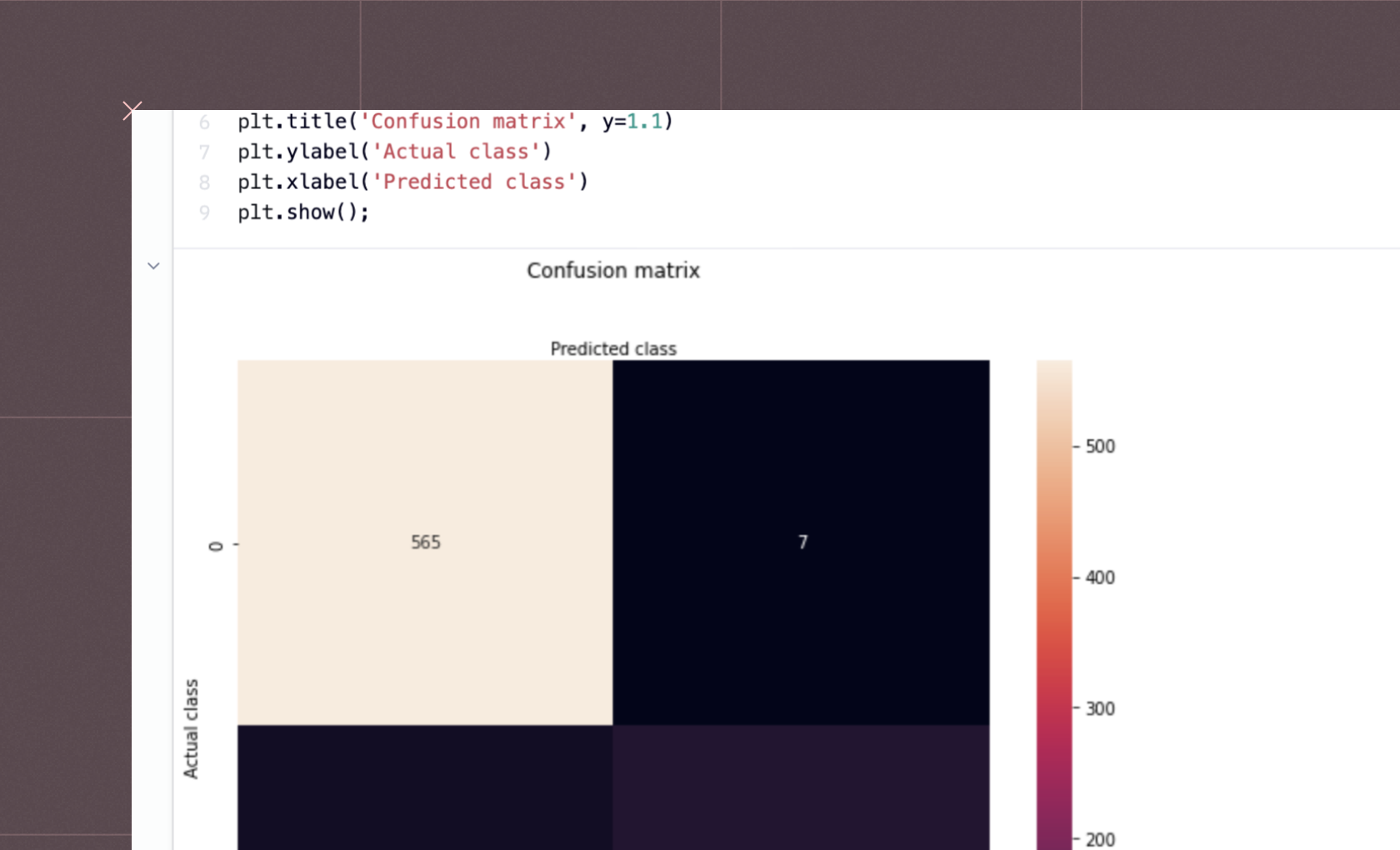
As you can see, we have obtained the higher values for all these measures which indicates that our model is performing quite well. Here are the details for each metric:

• Precision: 0.868. This means that out of all the points that our model labeled as outliers, about 86.8% of them were actually outliers.

• Recall: 0.92. This means that our model was able to correctly identify 92% of all the actual outliers in the data.

• F1 Score: 0.893. The F1 score balances precision and recall and is especially useful if you think it's equally important to minimize false positives and false negatives. In our case, the F1 score is high, suggesting that the model is performing well.

Visualize the Predicted Outliers

Now, let's make another scatter plot, but this time we'll color the points based on the model's predictions, so we can visualize what our model is doing. Hex makes this really easy to do— Instead of using matplotlib or seaborn, we can just use a Hex chart cell to get built-in interactivity. The created scatter plot will look something like this:

You might see that our model has predicted a lot of outliers correctly.

Once you are done with the coding part, you can head over to the App Builder section in the Hex environment. Here you might see that a dashboard was already created for you while you were doing the implementation. You are allowed to adjust the components of this dashboard by dragging and dropping them to the desired location. Once you are settled with all the changes, you can click on the Publish button to deploy the app with ease.

You have now created your own outlier detection system!

Best Practices for Outlier Detection

Outlier detection is a powerful tool, but it's important to use it wisely! Here's why following some best practices is crucial:

• Misidentified outliers can lead to misleading results. Mistaking normal data for outliers can skew your analysis and lead to incorrect conclusions.

• Not all outliers are bad. Sometimes, outliers can be valuable insights or indicate interesting discoveries.

Here are 5 key best practices to keep in mind for effective outlier detection:

• Understand Your Data: Before diving into detection methods, get familiar with your data. Explore summary statistics, visualizations (like boxplots), and domain knowledge to understand the expected range and distribution of your data. This helps you choose appropriate methods and avoid flagging normal variations as outliers.

• Consider Multiple Methods: Don't rely solely on one method. Try different techniques (statistical, distance-based, or machine learning) and compare the results. This can help you gain a more comprehensive understanding of potential outliers and avoid biases inherent in any single method.

• Visualize Your Outliers: Don't just rely on numbers. Use scatter plots, boxplots, or other visualizations to see how outliers are positioned compared to the rest of the data. This can help you identify patterns or clusters that might be missed by purely statistical methods.

• Context Matters: Outliers might not always be bad! Investigate flagged outliers in the context of your domain knowledge. For instance, a high sales figure might be an outlier statistically, but if it's due to a legitimate marketing campaign, it shouldn't be removed.

• Validate Results: After performing outlier detection, it is essential to validate the results to ensure their accuracy and reliability. This may involve cross-validation, comparing results with ground truth or expert knowledge, and assessing the impact of outliers on subsequent analyses or modeling tasks. Validating outlier detection results helps identify potential errors or inconsistencies and provides confidence in the findings.

By implementing these techniques and principles, you can enhance the accuracy and reliability of your data analysis processes, leading to more informed decision-making and actionable insights. Armed with this knowledge, you are well-equipped to tackle outlier detection challenges and unlock the hidden potential within your data.